Introduction to Logistic Regression

This Summer 2016 Release BigML is bringing Logistic Regression to the Dashboard, a very popular supervised Machine Learning method for solving classification problems. This upcoming release is the perfect scenario to guide you through Logistic Regression step by step. That is why we are presenting several blog posts to introduce you to this Machine Learning method.

Within this first post you will have a general overview of what Logistic Regression is. In the coming days, we will be complementing this post with five more entries: a second post that will take you through the six necessary steps to get started with Logistic Regression, a third post about how to make predictions with BigML’s Logistic Regression, a fourth blog post about how to create a Logistic Regression using the BigML API and a fifth one that will explain the same process using WhizzML instead, and finally, a sixth post that will analyze the difference between Logistic Regression and Decision Trees.

Let’s get started with Logistic Regression!

Why Logistic Regression?

Before machine learning hit the scene, the go-to tool for statistical modelling was regression analysis. Regressions aim to model the behavior of an objective variable  as a combination of effects from a number of predictor variables. Among these tried-and true techniques is Logistic Regression, which was originally developed by statistician David Cox in 1958. Logistic regression is used to solve classification problems, where the objective is a categorical variable. Let’s see a simple example.

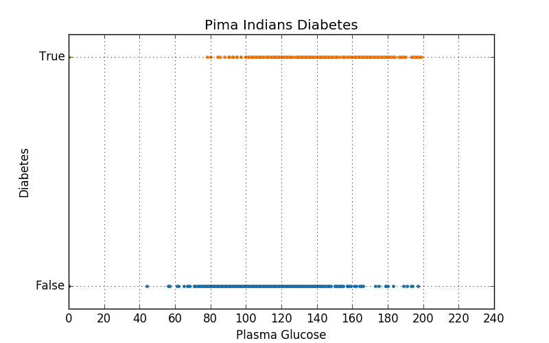
The dataset we’ll work with contains health statistics from 768 people belonging to the Pima Native American ethnic group. Our objective is to model the effect of an individual’s plasma glucose level on whether that individual contracts diabetes. The above scatterplot shows the plasma glucose levels of individuals with and without diabetes. At a glance, we can see that some relationship exists, where higher levels of plasma glucose are indicative of having diabetes. Note that while the x-axis is numeric in the scatterplot, the y-axis is categorical. This means we’ll need to apply a transformation before we can encode this relationship numerically. Rather than relating glucose levels directly to true/false values, we model the probability of diabetes as a function of plasma glucose. Speaking in terms of probability is appropriate because, as we can see in the above graph, there is no clear-cut threshold on plasma glucose beyond which we can say a person will have diabetes. Most individuals with plasma glucose below 80 mmol/L do not have diabetes, while most with levels above 180 mmol/L have diabetes. Within that range however, there is a significant amount of overlap. We need a way to express this interval of fuzziness flanked by two zones of certainty. For this purpose, we’ll use a function called the logistic function.

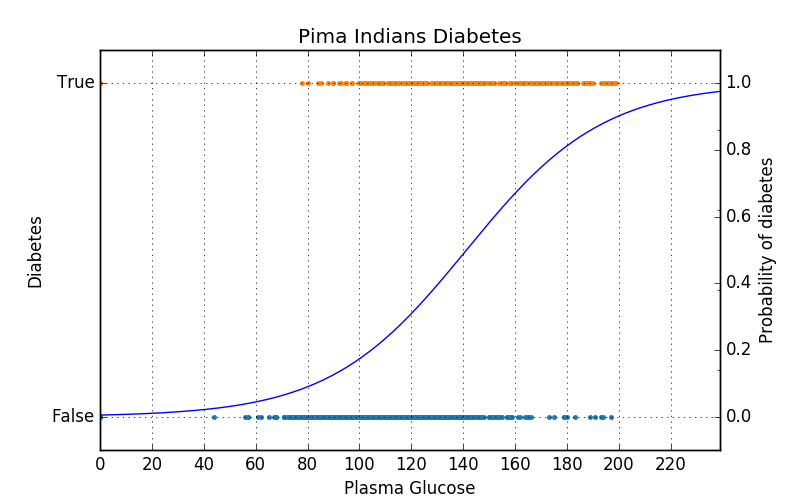
In this single-predictor example, our regression function is characterized by only two parameters: the slope of the transition and where the transition point is located along the x-axis. Fitting a logistic regression is simply learning the values of these parameters. The ability to encapsulate the model in only two numbers is one of the main selling points of logistic regression. Check out these slides from the Valencian Summer School in Machine Learning 2016 for more details and examples.

Having said that, in this first post we won’t go too deep into Logistic Regression. Sometimes simplicity is the key to understand the basic concepts:

• The aim of a Logistic Regression is to model the probability of an event that occurs depending on the values of the independent variables.

• A Logistic Regression estimates the probability that an event occurs for a randomly selected observation versus the probability of this event not occurring at all.

• A Logistic Regression classifies observations by estimating the probability that an observation is in a particular category.

These videos from Brandon Foltz offer a deeper dive into the essence of Logistic Regression:

Want to know more about Logistic Regression?

Check out our release page for documentation on how to use Logistic Regression with the BigML Dashboard and the BigML API. You can also watch the webinar, see the slideshow and read the other blog posts of this series about Logistic Regression.