BigML is bringing Logistic Regression to the Dashboard so you can solve complex classification problems with the help of powerful visualizations to inspect and analyze your results. Logistic Regression is one of the best-known supervised learning algorithms to predict binary or multi-class categorical values such as “True/False”, “Spam/ Not Spam”, “Offer A / Offer B / Offer C”, etc.
In this post we aim to take you through the 6 necessary steps to get started with Logistic Regression:

1. Uploading your Data
As usual, start by uploading your data to your BigML account. BigML offers several ways to do it, you can drag and drop a local file, connect BigML to your cloud repository (e.g., S3 buckets) or copy and paste a URL. BigML automatically identifies the field types. Field types and other source parameters can be configured by clicking in the source configuration option.
2. Create a Dataset
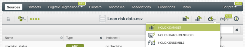
From your source view, use the 1-click dataset option to create a dataset, a structured version of your data ready to be used by a Machine Learning algorithm.
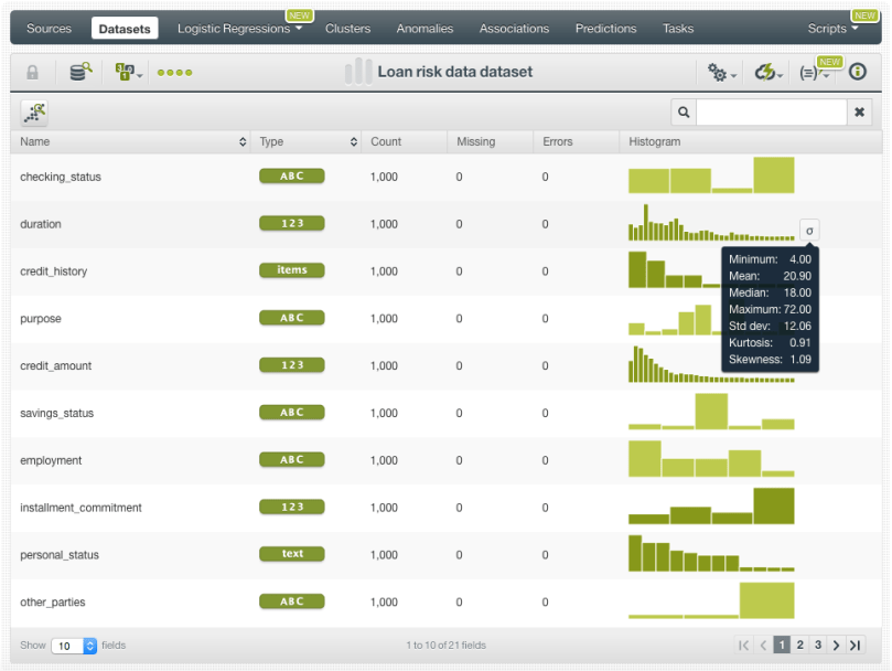
In the dataset view you will be able to see a summary of your field values, some basic statistics and the field histograms to analyze your data distributions. This view is really useful to see any errors or irregularities in your data. You can filter the dataset by several criteria and create new fields using different pre-defined operations.
Once your data is clean and free of errors you can split your dataset in two different subsets: one for training your model, and the other for testing. It is crucial to train and evaluate your model with different data to ensure it generalizes well against unseen data. You can easily split your dataset using the BigML 1-click option, which randomly sets aside 80% of the instances for training and 20% for testing.

3. Create a Logistic Regression
Now you are ready to create the Logistic Regression using your training dataset. You can use the 1-click Logistic Regression option, which will create the model using the default parameter values. If you are a more advanced user and you feel comfortable tuning the Logistic Regression parameters, you can do so by using the configure Logistic Regression option.


Find below a list containing a brief summary for each of the configuration parameters. If you want to learn more about them please check the Logistic Regression documentation .
-
Objective field: select the field you want to predict. By default BigML will take the last valid field in your dataset. Remember it must be categorical!
-
Default numeric value: if your numeric fields contain missing values, you can easily replace them by the field mean, median, maximum, minimum or zero using this option. It is inactive by default.
-
Missing numerics: if your numeric fields contain missing values but you think they have a meaning to predict the objective field, you can use this option to include them in the model. Otherwise, instances with missing numerics will be ignored. It is active by default.
-
Eps: set the value of the stopping criteria for the solver. Higher values can make the model faster, but they may result in a poorer predictive performance. You can set a float value between 0 and 1. It is set to 0.0001 by default.
-
Bias: include or exclude the intercept in the Logistic Regression formula. Including it yields better results in most cases. It is active by default.
-
Auto-scaled fields: automatically scale your fields so they all have the same magnitudes. This will also allow you to compare the field coefficients learned by the model afterwards. It is active by default.
-
Regularization: prevent the model from overfitting by using a regularization factor. You can choose between L1 and L2 regularization. The former usually gives better results. You can also tweak the inverse of the regularization strength.
-
Field codings: select the encoding option that works best for your categorical fields. BigML will automatically transform your categorical values into 0 -1 variables to support non-numeric fields as inputs, which is a method known as one-hot encoding. Alternatively, you can choose among three other types of codings: dummy coding, contrast coding and other coding. You can find a detailed explanation of each one in the documentation.
-
Sampling options: if you have a very large dataset, you may not need all the instances to create the model. BigML allows you to easily sample your dataset at the model creation time.
At this point you may be wondering… ok, so which parameter values should I use?
Unfortunately, there is not a universal response for that. It depends on the data, the domain and the use case you are trying to solve. Our recommendation is that you try to understand the strengths and weaknesses of your model and iterate trying different features and configurations. To do this, the model visualizations explained in the next point play an essential role.
4. Analyze your Results
When your Logistic Regression has been created you can use BigML’s insightful visualizations to dive into the model results and see the impact of your features on model predictions. Take into account that most of the time, the greatest gains on performance come from feature selection and feature engineering, which can be the most time consuming part of the Machine Learning process. Analyzing the results carefully, and inspecting your model to understand the reasons behind the predictions is key in further validating the findings in contrast to expert opinion.
BigML provides a 1D and 2D chart and the coefficient table to analyze your results.
1D and 2D Chart
The Logistic Regression chart provides a visual way to analyze the impact of one or more fields on predictions.
For the 1D chart you can select one input field in the x-axis. In the prediction legend to the right, you will see the objective class predictions as you mouse over the chart area.

For the 2D chart you can select two input fields, one per axis and the objective class predictions will be plotted in the color heat map chart.
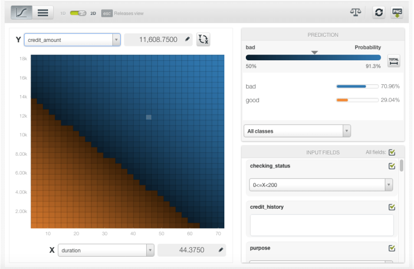
By setting the values for the rest of input fields using the form below the prediction legend, you will be able to inspect the combined interaction of multiple fields on predictions.
Coefficients table
BigML also provides a table to display the coefficients learned by the Logistic Regression. Each coefficient has an associated a field (e.g., checking_status) and an objective field class (e.g., bad, good etc.). A positive coefficient indicates a positive correlation between the input field and the objective field class, while a negative coefficient indicates a negative relationship.

To find out more about the interpretation of the Logistic Regression chart and coefficient table results, follow our next blog post of this series: Predicting Airbnb Prices with BigML Logistic Regression.
5. Evaluate the Logistic Regression
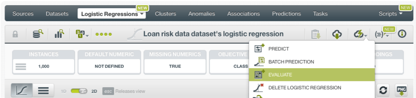
Like any supervised learning method, Logistic Regression needs to be evaluated. Just click on the evaluate option in the 1-click menu and BigML will automatically select the remaining 20% of the dataset that you set aside for testing.
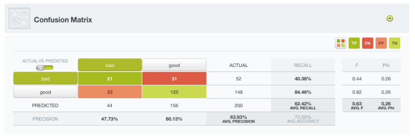
The resulting performance metrics to be analyzed are the same ones as for any other classifier predicting a categorical value.
You will get the confusion matrix containing the true positives, false positives, true negatives and false negatives along with the classification metrics: precision, recall, accuracy, f-measure and phi-measure. For a full description of the confusion matrix and classification measures see the corresponding documentation.
Rinse and repeat! As we mentioned at the end of step 3, repeat steps from 3 to 5 trying out different configurations, different features, etc. until you have a good enough model.
6. Make Predictions
When you finally reach a satisfying model performance, you can start making predictions with it. In BigML, you can make predictions for a new single instance or multiple instances in batch. Let’s take a quick look to both of them!
Single predictions
Click in the Predict option and set the values for your input fields.
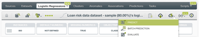
A form containing all your input fields will be displayed and you will be able to set the values for a new instance. At the top of the view you will see the objective class probabilities changing as you change your input field values.

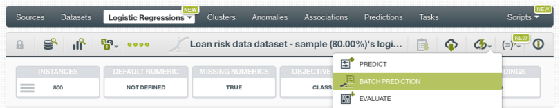
Batch predictions
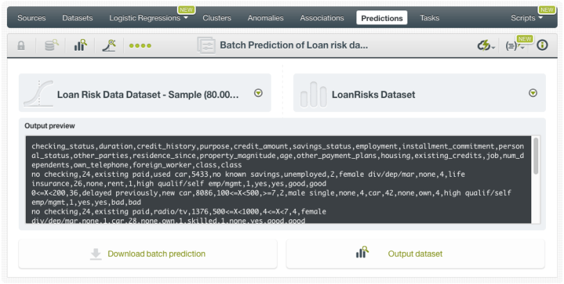
Use the Batchprediction option in the 1-click menu and select the dataset containing the instances for which you want to know the objective field value.
You can configure several parameters of your batch prediction like the possibility to include all class probabilities in the batch prediction output dataset and file. When your batch prediction finishes you will be able to download the CSV file and see the output dataset.
In the next post we will cover a real use case using Logistic Regression to predict Airbnb prices to delve into the Logistic Regression results interpretation.
If you want to learn more about Logistic Regression please visit our release page for documentation on how to use Logistic Regression with the BigML Dashboard and the BigML API. You can also watch the webinar, see the slideshow, and read the other blog posts of this series about Logistic Regression.
