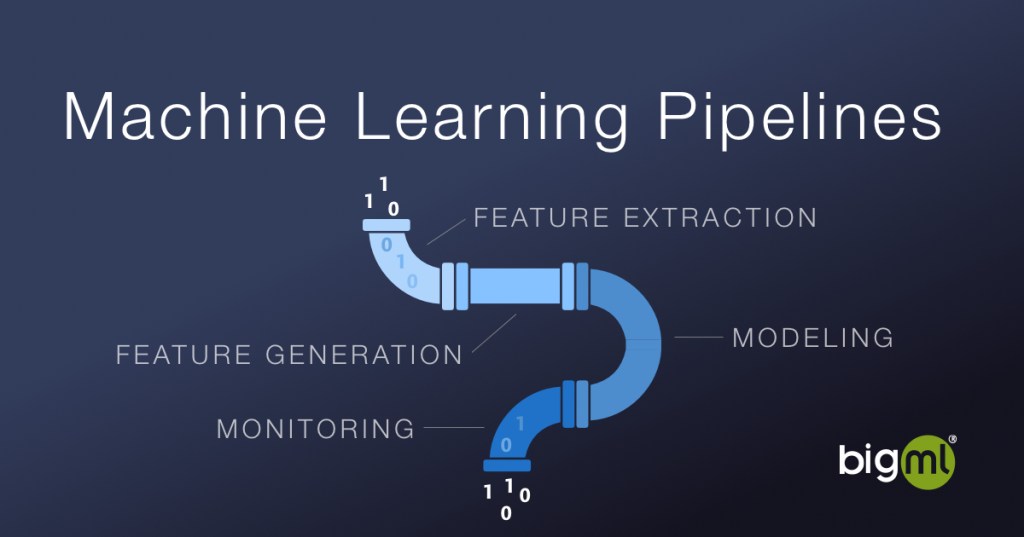
As Machine Learning solutions to real-world problems spread, people are beginning to acknowledge the glaring need for solutions that go beyond training a single model and deploying it. The simplest process should at least cover feature extraction, feature generation, modeling, and monitoring in a traceable and reproducible way. In BigML, it’s been a while since we realized that, and the platform has constantly added features designed to help our users easily build both basic and complex solutions.
Those solutions often need to be deployed in particular environments. Our white-box approach is totally compatible with that, as users can download the models created in BigML and predict with them wherever needed by using bindings to Python or other popular programming languages. But what about the features and transformations that your Data Scientists used to create the training datasets for those models? We need more than the model information for that. In fact, we need to reproduce the same sequence of steps that were used before building the model: we need a transformations Pipeline. This post will explain how that’s automatically obtainable by using BigML and its Python bindings.
Do we really need Pipelines?
Just to set an example showing the need for some kind of encapsulation of the steps used before modeling, let’s recall the Predicting Stock Swings with PsychSignal, Quandl, and BigML blog post that we wrote years ago. The goal was to use both stock data plus the general sentiment that people associated with that stock to try to predict the swing of the stock with respect to the median. In this case, we will simplify the goal and we will try to predict whether a stock price will go up or down during the training day. The original data looks like this:
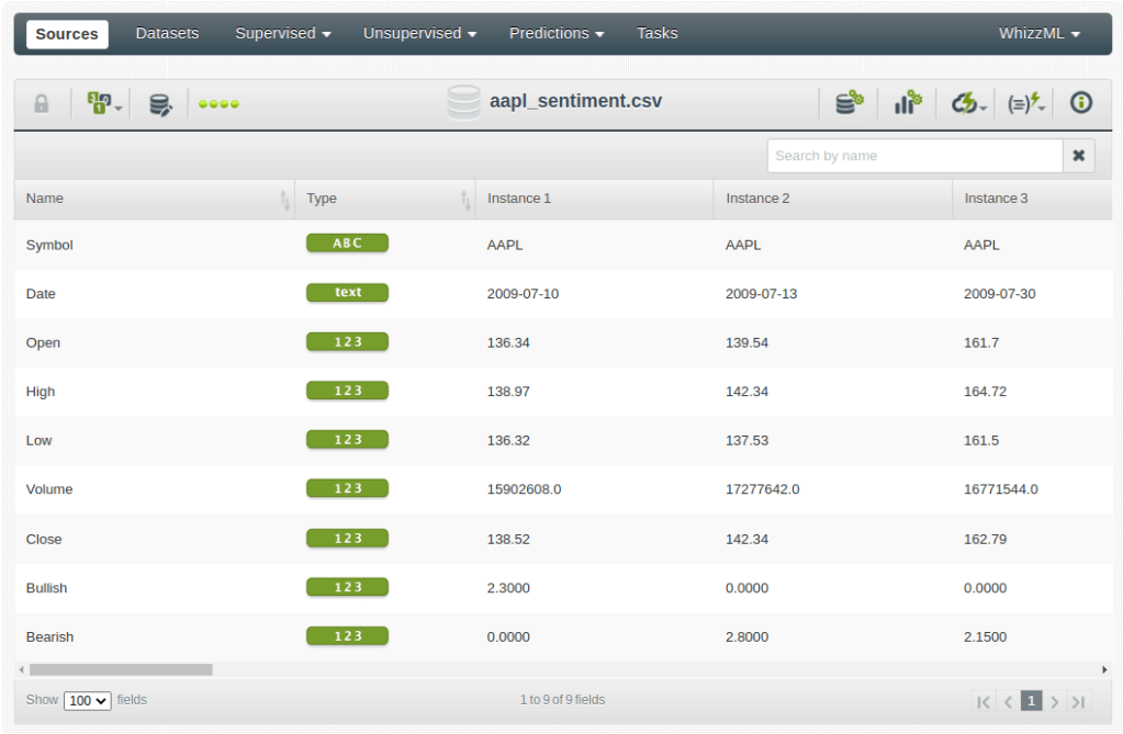
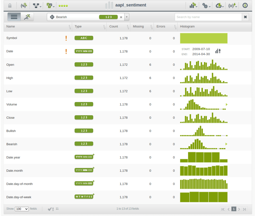
It contains information about the daily stock trade prices and volumes, plus a couple of fields that store the sentiment associated with the stock during the day (i.e., Bullish/Optimist, Bearish/Pessimist). When uploaded to BigML, the resulting dataset is extended by some extracted features: the date-time field decomposition.
The generated fields are new features that could be used by the algorithm too. If that’s the case, a similar extraction should be applied to any new test data before being run through the model to get predictions from it correctly. That’s the first transformation that should be reproduced for your raw test data when predicting.
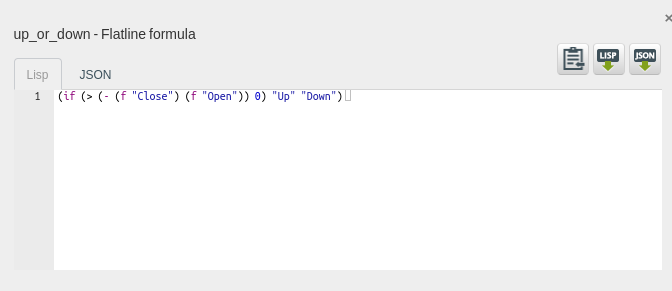
In addition, we realize that the problem at hand is predicting a field that cannot be found in the raw data. Instead, it needs to be produced as a combination of them. In BigML, that combination should be defined by using our transformations language, Flatline, to generate the expression that we’re interested in and store the result in a new up_or_down generated field.
Also, as explained in the referred post, the model needs to be based on the previous days’ values. Possible input fields could be the previous day’s Open and Close values (Open-1 and Close-1) or even the mean value across a time window (like the previous five days) or others described in another of our posts on Financial Analysis. Again, these are new fields that can be added using the corresponding Flatline expressions, and the process will generate a new extended dataset. Finally, after some sequence of transformations on the original data, the final dataset used to train the model might have additional fields like these:

Obviously, the same operations should be applied to any new test data row to get ready for the prediction function. Those transformations then become the new steps of a Pipeline to be applied to input data at prediction time.
BigML’s Pipelines
The BigML Python bindings have been offering classes that download and use locally any kind of model built in the BigML platform. As an example, this is the code snippet that you would need to use a particular model to produce predictions, provided that the original raw data was used to train the model.
from bigml.supervised import SupervisedModel
local_model = SupervisedModel("model/637695b5bd91a97d540102c9")
The SupervisedModel class downloads the JSON that defines the patterns of a particular Supervised Model and offers a .batch_predict method to apply it to test data rows that have the original data fields.
input_data = [{"Bullish": 2.3, "Bearish": 0.2},
              {"Bullish": 0.12, "Bearish": 4.3}]
local_model.batch_predict(input_data)
However, in the previous section’s example, the model was trained using additional fields derived from the original ones. Therefore, we need information about the transformations that have been applied to create those fields for any test data row. How can we do that? Similar to what we saw for models and thanks to BigML‘s traceable resources, we can retrieve the information from the datasets that contain those transformations. The transformations will become steps in a Pipeline. BMLPipeline is the right class to do that.
from bigml.pipeline.pipeline import BMLPipeline
pipeline = BMLPipeline("swing", "dataset/637695aebd91a97d540102c6")
The BMLPipeline class needs a unique name and a dataset ID (it could also be a model ID or even a list of them, but let’s discuss that later) as arguments. On instantiation, it will create a folder in your current directory named after the name that you provided for the Pipeline itself. Each dataset found in the backtrace from the dataset used as the argument to the original data will then be downloaded and analyzed. A new transformation step will be added to the Pipeline as needed. When instantiating the BMLPipeline on a training dataset, the generated Pipeline will contain all the transformations that were made to achieve the training dataset fields. Every Pipeline offers the .transform method that receives the list of new input data to which the transformations should be applied and adds the transformed fields subsequently. The resulting data will then have the right input fields for the model to be able to apply its rules and produce predictions as expected.
import csv
raw_data = []
with open("test_data.csv") as test_file:
    reader = csv.DictReader(test_file)
    for row in reader:
        raw_data.append(row)
input_data = pipeline.transform(raw_data)
Advanced Pipelines
As explained in this post’s preface, the previous example still lacks an important part of any real-world Machine Learning solution: model monitoring. A good strategy to decide if a model becomes outdated is building an anomaly detector using the model’s training data. Then, the model can be used to get a prediction and the corresponding anomaly detector to assign an anomaly score to every test data row. If the score is too high, that test data row might be an outlier, and the model’s prediction for it should not be trusted blindly. Also, if the distribution of scores drifts to the higher range for a significant amount of test data, that might be indicating that the model is becoming outdated and needs retraining.
In both cases, we can think of the model and the anomaly detector as generators for a new set of fields: the prediction and the anomaly score. We will base our reasoning and our decisions on them as well as on the original data and the training dataset transformations. From that point of view, both the model .predict method and the anomaly detector .anomaly_score method can be regarded as additional transformation steps in a Pipeline. To use them as such, you’ll just need to instantiate a BMLPipeline using their IDs.
from bigml.pipeline.pipeline import BMLPipeline
pipeline = BMLPipeline("ml_solution",
                       ["model/637695b5bd91a97d540102c9",
                        "anomaly/637695b9d63708290e011fad"])
By calling the .transform method, new fields will now be included in every test data row containing the prediction of the model, its probability, and the anomaly score generated by the detector. That information can then be used to monitor, use or discard the model’s predictions.
>>> import pandas as pd
>>> dataframe = pd.read_csv("data/csco_sentiment.csv")
>>> ml_solution_output = pipeline.transform(dataframe)
    Symbol        Date   Open  ...    prediction  probability    score
0     CSCO  2009-10-12  24.07  ...  Under median     0.699561  0.81265
1     CSCO  2009-10-13  23.58  ...   Over median     0.694969  0.58955
2     CSCO  2009-10-15  24.25  ...  Under median     0.688034  0.56721
3     CSCO  2009-11-04  23.31  ...  Under median     0.544574  0.56613
4     CSCO  2009-11-05  24.05  ...  Under median     0.544574  0.55675
..     ...         ...    ...  ...           ...          ...      ...
881   CSCO  2014-04-23  23.52  ...  Under median     0.958333  0.43843
882   CSCO  2014-04-24  23.64  ...  Under median     0.958333  0.44242
883   CSCO  2014-04-28  23.15  ...  Under median     0.958333  0.44475
884   CSCO  2014-04-29  23.20  ...  Under median     0.958333  0.42830
885   CSCO  2014-04-30  23.08  ...  Under median     0.958333  0.45008

[886 rows x 34 columns]
There are more options and transformations that can be applied using the BMLPipeline and its generic Pipeline class, indeed. Pipelines can be composed, as each one can be regarded as a transformation, which can become a new Pipeline step. That opens up many possible combinations to enrich your data with BigML and the highly versatile Python language. This represents one more step towards sensible data-driven decision-making using BigML. One last thing: there’s more to come on this topic, so stay tuned!
