With regards to the analysis of financial markets, there exists two major schools of thought: fundamental analysis and technical analysis.

• Fundamental analysis focuses on understanding the intrinsic value of a company based on information such as quarterly financial statements, cash flow, and other information about an industry in general. The goal is to discover and acquire assets that are currently undervalued, often with a long-term approach to investing.
• Technical analysis is based on the assumption that all of the relevant information about a company is already baked into its share price. Rather than financial statements, this analysis is focused on analyzing trends in the share price in order to forecast the future value, and can often be conducted on extremely short time scales.

While both strategies clearly rely on data, the type of data that is most useful and relevant is drastically different. In this blog post, we will explore how sliding window transformations and dataset joins are fundamental data transformation operations for technical and fundamental financial analysis, respectively.

Loading and Filtering Data

In this use case, we will demonstrate how the exploration of market data is enabled by quick and easy data transformations using BigML. We will be using two primary datasets that contain stock market data from 2016. This data, originally obtained from Kaggle, was pre-processed so as to be more relevant for the new BigML transformation options being highlighted. You can access both of these updated datasets in the BigML Gallery.

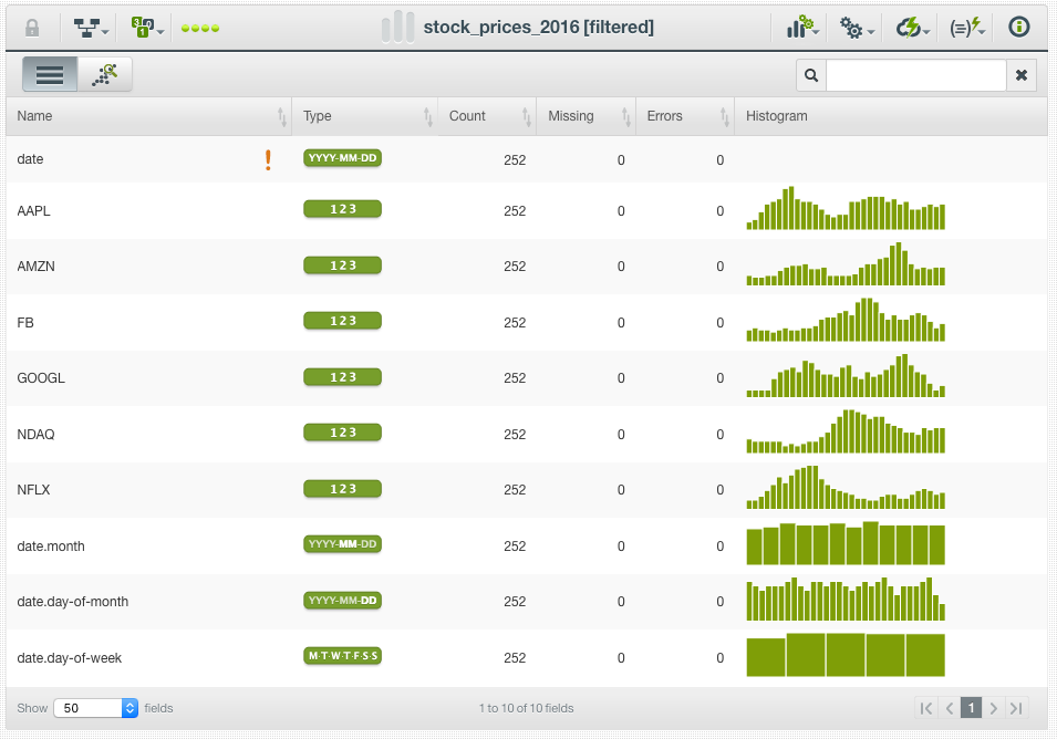
To scope down the problem, we are including only the NASDAQ Index and “FAANG” stocks. These stocks correspond to high market cap tech sector companies including Facebook (FB), Amazon (AMZN), Apple (AAPL), Netflix (NFLX), and Alphabet (GOOGL).

Time Series Feature Engineering

Time series data may not appear to be feature rich at first glance. For example, for each stock in this dataset (e.g. AAPL), a single vector of values exists representing the closing price of the asset for each day. Without further analysis or additional data, this is unlikely to be useful for any sort of forecasting task. Of course, there is a reason why technical analysts spend a lot of time evaluating data visually: they are looking to identify past, ongoing, and emerging trends within the time series. Fortunately, these visual trends can also be systematically created and categorized through feature engineering, a task that rather simple data transformations are able to accomplish en masse.

One of the most valuable classes of data transformations for time series data is that of sliding windows. BigML now supports a large number of sliding window transformations, including measurements of central tendency (mean and median), computation of sums, products, or differences within a window, and returning maximum or minimum values. The parameters needed for a sliding window computation consist of only the desired operation and the start and end of the window relative to the reference instance. Typically only historical data would make intuitive sense for a time series forecasting problem. However, sliding windows can also be computed using future values if desired. For the sake of example, we will highlight two useful and often-employed types of transformations:

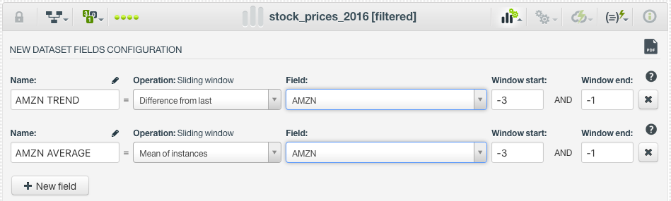
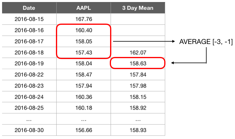
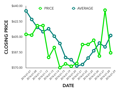
• Mean of instances: this transformation calculates the average value in a window. This type of transformation can be very useful for smoothing out noisy data in order to focus on more sustained trends.

• Difference from last: this transformation essentially determines a local, recent trend in the direction of the data. In financial applications, this is frequently referred to as the “momentum” and it represents the velocity of price changes.

Joining Data Sources

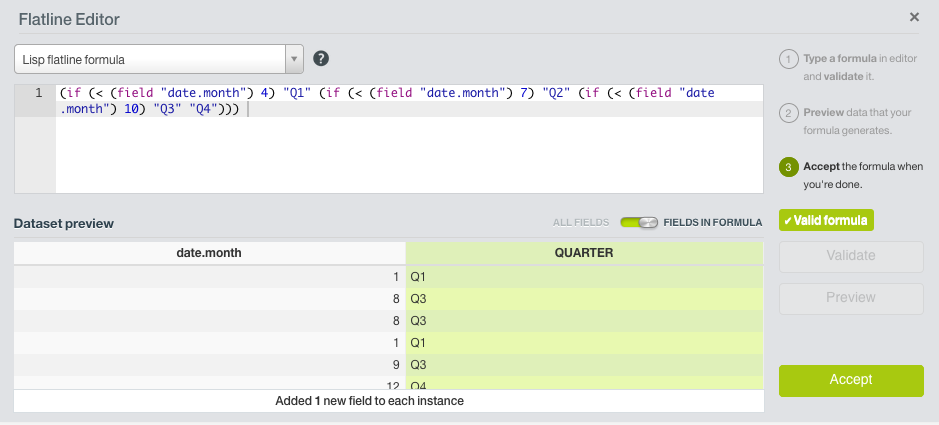
As introduced previously, fundamental analysis is not nearly as concerned with trends in time series as it is with understanding the intrinsic value of a company through additional sources of information. Accordingly, the most powerful data transformation for a fundamental analysis is the ability to quickly and accurately join together information sourced from disparate data sources. Because fundamental financial data is often issued on a quarterly basis, we first will add an additional field to our dataset that assigns each instance to a quarter, based on the month of the year.

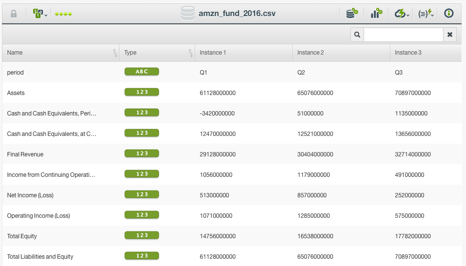
We will then add a new dataset consisting of fundamental data from Amazon to our Dashboard. The instances in this dataset refer to quarters rather than individual dates, and include additional fields useful for fundamental analysis such as operating income, revenue, and total equity.

What would be most useful is to be able to join this fundamental data with the information we already have regarding the stock price values. This type of operation is known as a join and can now be conducted in the BigML Dashboard without needing to know or utilize SQL, Pandas, Tableau or other data manipulation tools. The fields “period” and “QUARTER” respectively refer to the same information, and allow the associated fundamental analysis to be added to each instance of the daily closing price of Amazon.

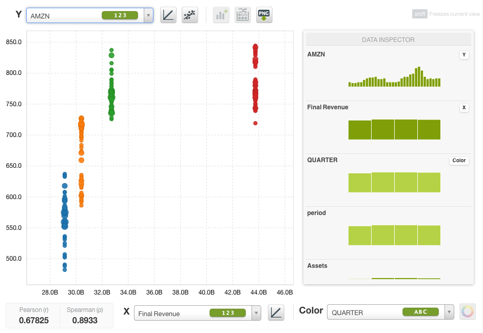
The resulting dataset allows for more intricate visualizations and association discovery than possible with only time series or fundamental data. Using the scatterplot option in the Dashboard, we can view the range of closing prices for this stock in relation to fundamental analysis variables, such as “Final Revenue”, as shown below. In the case of Amazon in 2016, there appears to be a strong correlation between these variables although it is far from telling the entire story with regards to price forecasting.

This blog post shows the power of transforming and combining data in order to gain powerful insights about seemingly simple datasets. In particular, sliding windows and dataset joins are frequently used to perform financial analysis of the technical and fundamental variety. We encourage you to dig deeper into this dataset to find unique and informative insights that can be uncovered.

Want to know more about Data Transformations?

If you have any questions or you would like to learn more about how Data Transformations work, please visit the release page. It includes a series of blog posts, the BigML Dashboard and API documentation, the webinar slideshow, as well as the full webinar recording.