No-Code Object Detection: Easily Tackling Image Data-Driven Use Cases

BigML will release Object Detection on Tuesday, June 28, 2022! This feature is a significant capability on top of image classification. While image classification determines whether an image belongs to a certain class, Object Detection goes further. It not only shows where an object is in the image, but it also can show where instances of objects from multiple classes are located in the image. Because of this, the use cases for Object Detection are broader than for simple classification or regression. The following is an example to show how, with just simple point-and-click actions on the BigML Dashboard, anyone can do “no-code” Object Detection!

Let’s build an Object Detection model that can detect cats and dogs. We collected pictures of cats and dogs, some of which are from the popular Pascal-VOC dataset. We also downloaded many pictures from the Internet, and others we took ourselves. 

Annotating the Data

We zipped 288 pictures and uploaded them to the Dashboard. This created an image composite source which has image and path fields. 

First, we need to annotate the training data. Annotation means marking what objects are where in the images. We draw a bounding box around an object and add its class label. In BigML, there is a dedicated field type called regions for this. BigML’s image composite sources provide an annotation interface. In the composite source “cats-dogs.zip” we just created, go to its “Images” view and click on the “+” to add a new label field. Then, we name the new field “boxes”, and select the field type “Regions” from the dropdown list.

Now we can click on an image to bring out the annotation interface:

We create two class labels, “cat” and “dog”. Select one class, and then draw a rectangular box to surround an object in the image. We draw the box by first clicking a point in the image as a vertex of the rectangle, and then clicking another point as its opposing diagonal vertex. When clicking the first point, the crosshair is very useful for estimating the coverage of the rectangle. 

After finishing the drawing, it also labels the image as the class we selected. 

We can edit the box by clicking on the editing icon on the right or (SHIFT+E). We can move the box or change its size, or delete it and start over. 

There are other options to make the annotation easier and quicker. We can hide the class labels, we can also hide certain or all classes so that it’s easier to see an object when drawing. We can copy regions to the next image, either manually or automatically, which is very useful when annotating images that have similar objects, or even images similar to each other such as video frames. Once we finish drawing regions on all objects in an image, we click on “Save regions” to save the annotation.

After we have annotated all the images, we are ready to create a dataset.

Creating Datasets

While we use image composite sources for annotating data, the datasets are the true launch pads for Machine Learning in BigML – all models are created from datasets. We create a dataset from annotated composite source “cats-dogs.zip” by clicking on the 1-click dataset option in the cloud action menu.

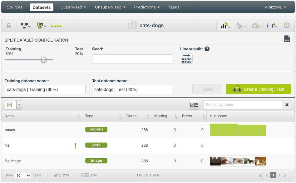
As with any other datasets in BigML, after creation, we can see its field summaries, some statistics, and field histograms. 

As shown above in the field table in the dataset view, the regions field “boxes” was assigned as the objective field automatically. The histogram of the regions field shows the distribution of the classes, which indicates that there are slightly more cats than dogs in the dataset.

The red exclamation point indicates that “file” is set to non-preferred automatically, which means it won’t be used when training a model. There are 288 images with no missing values or errors. In the histogram of the image field are mini previews of the images, which can be changed by clicking on the refresh button.

Before we create a model, we can split the dataset into two datasets so that we can use one to train models while using the other for evaluation. BigML provides a 1-click “Training|Test Split” option, which randomly sets aside 80% of the instances for training and 20% for testing.

Creating a Model

Deepnet is the BigML resource for deep neural networks. When creating a Deepnet from a dataset with a regions field as its objective field, it will train a convolutional neural network (CNN) as the Object Detection model.

From the training dataset “cats-dogs | Training [80%]”, we use the 1-click Deepnet option from the cloud action menu to create a Deepnet using default parameter values. 

Object Detection is computationally harder than image classification in general, so the Deepnet training may take more resources and take longer time to finish. But don’t worry, with the BigML backend and GPU-supported servers, it’s still a breeze compared to other tools. When the training finishes, we are at the Object Detection Deepnet page:

We can see lots of useful information about the Object Detection Deepnet, its parameters, as well as its precision, recall and F-measure. The main focus of the page is the performance from a set of sampled instances. This set is called the holdout set and was used during the Deepnet training for validation. On the right, in the performance panel, it shows that there are 66 objects in the holdout set. In that holdout set, 45 objects are predicted correctly and 21 are not. The class list shows two classes and their recall rates, respectively. For instance, there are 35 cats, 24 of them are predicted correctly. Clicking on a class will change all performance data for both cats and dogs, to the specific class. Use the reset button next to the title “Deepnet Performance” to reset it back to overall performance. For instance, clicking on the “cat” class:

The images in the holdout set are divided into two sections. The top section lists all images in which all objects are predicted correctly. The bottom section lists all images in which at least one object is predicted incorrectly. We can easily glimpse the predicted regions in all images. Each section shows up to 6 images and can be scrolled using the arrow buttons beneath. Clicking on an image, we get a closeup view of its prediction results:

By default, it shows the correctly predicted regions and their scores, as indicated by the highlighted checkbox on the right. We can also select the “Correctly identified regions” checkbox to show the ground truth regions. Ground truth regions are the regions that were annotated earlier and properly surround the objects. We can compare the prediction regions and ground truth regions and see how they overlap each other.

In this particular image, both objects were predicted correctly, so there are no incorrectly identified regions, nor incorrectly predicted regions. We can also hide a class of objects using the label buttons on the top right. 

If we click on an image in the bottom section, for example:

There are two correctly predicted regions in this image, but there are actually three cats. We can compare the predicted and ground truth regions by selecting also the “Correctly identified regions” checkbox:

Or we can just view all ground truth regions by unselecting the “Correctly predicted regions” checkbox and selecting both “Correctly identified regions” and “Incorrectly identified regions” checkboxes:

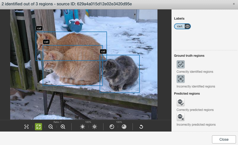
With these checkbox combinations, it’s clear that the model missed the cat in the back. It’s largely due to the fact that much of the cat in the back is blocked by the cat in the front.

Evaluating the Model

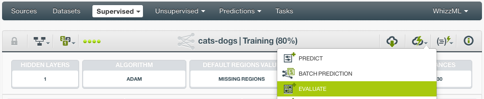
While the holdout set gives a good insight into how good a Deepnet predicts regions, it is not an actual evaluation. In order to measure the Deepnet’s true performance (how good it is at predicting regions not seen in training) we need to create an Object Detection evaluation. Go to the cloud action menu, click on “EVALUATE”, 

Then we will see:

Our test dataset is the one we split from the original dataset and it has 58 instances, 20% of the 288 images. We click on the “Evaluate” button to create an evaluation:

To calculate the correctness of an Object Detection, we use the IOU threshold, Intersection over Union. As the name suggests, it is a ratio of the area of intersection over the area of union between the ground truth and predicted regions. It measures how much overlap there is between the ground truth and predicted regions and hence how accurate the prediction is. We can pick one of three IOU thresholds 0.5, 0.75, or 0.9 by clicking on the IOU tabs on top. The IOU determines how good a prediction has to be, in order to be called correct. The default is 0.5. All other metrics are calculated based on the selected IOU. Naturally, when the IOU is high, such as 0.9, there are fewer correct predictions, thus the performance under 0.9 IOU is much lower than that under 0.5 IOU.

On the right, we can see summary metrics for the evaluation: the numbers of true positives, false positives and false negatives, precision, recall, F1-Score, and so on. On the left is the graph of Precision-Recall AUC (Area Under the Curve). There are two icons above the graph, one is to show the area under the convex hull (AUCH), and another to export the graph.

All evaluation metrics are with regard to a specific class, and we can use the object class dropdown to select a different class. There is a “Score Threshold” slider to filter the prediction score, which is a product of the probability of the object belonging to the class and the probability of the region containing the object. Lowering the threshold will increase the true positives hence improving the recall, but the precision suffers. And vice versa when increasing the threshold.

Under the metrics are sampled images from the test dataset. We can use the refresh button to load different images. We can also click on an image for closeup inspection, comparing the predicted regions and ground truth regions:

The layout described so far is under the “Class detail” view. We can click on the “Summary” tab to view all evaluation metrics in a tabular format, with all classes aggregated:

Making Predictions

The main goal to build a Machine Learning model is to make predictions. That is also true for Object Detection. From the Deepnet page, click on the “PREDICT” option from the cloud action menu:

This presents the “prediction form” of the Object Detection Deepnet we created, where we can select an uploaded image and predict it.

Once an image is selected, click on the “Predict” button to perform the prediction.

We can see the prediction results along with their scores. Again, a prediction score measures how confident the model is about the prediction. It’s the product of the probability of the predicted region containing an object and the probability of the object being the predicted class. We can get a closeup view of the prediction by clicking on the image:

Keep in mind that this is a new image without annotation, so there are no ground truth regions to compare with. The model did a great job predicting both objects, very accurately. We can use the “Score Threshold” slider to filter the predictions. For instance, if the threshold is increased to 70%, there will be only one object predicted:

Let’s try another image,

These predictions are even better, with 80%+ scores across the board.

If we want to predict two or more images, BigML Batch Prediction is the resource to use. The input to a batch prediction is a dataset. We put 8 images together, created a composite source, then a dataset called “batch”. From the Object Detection Deepnet page, click on the “BATCH PREDICTION” option on the cloud action menu:

We select the dataset “batch”, and configure output settings like in any other batch predictions as needed:

After the batch prediction is created, we can preview its sampled output including sampled images with predicted regions:

We can inspect the predictions by clicking on an image:

Summary

The applications of Object Detection are limitless. However, with the benefits come complexities that demand more computing resources be it software, hardware, GPUs, etc. But the BigML platform abstracts away those complexities. As shown by the example in this post, we collected enough images, uploaded them, and annotated them with regions and labels. Then we created datasets and trained a Deepnet to perform Object Detection. We also evaluated the model and used it to predict new images that detected objects accurately. All of these tasks were done on the Dashboard with a few clicks. This is as accessible as it gets in Machine Learning. And just as our motto suggests, BigML has made Object Detection beautifully simple for everyone.

Be sure to visit the release page of BigML Object Detection, where you can find more information and documentation.