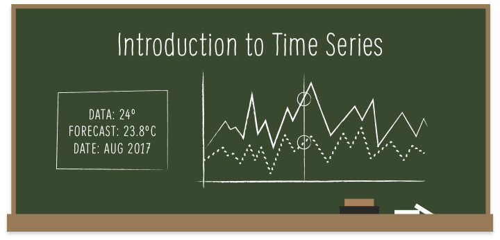
We are proud to present Time Series as a new resource brought to the BigML platform. On July 20, it will be available via the BigML Dashboard, API and WhizzML. Time Series is a sequentially indexed representation of your historical data that can be used to solve classification and segmentation problems, in addition to forecasting future values of numerical properties, e.g., air pollution level in Madrid for the last two days. This is a very versatile method often used for predicting stock prices, sales forecasting, website traffic, production and inventory analysis, or weather forecasting, among many other use cases.

Following our mission of democratizing Machine Learning and making it easy for everyone, we will provide new learning material for you to start with Time Series from scratch and become a power user over time. We start by publishing a series of six blog posts that will progressively dive deeper into the technical and practical aspects of Time Series with an emphasis on Time Series models for forecasting. Today’s post sets the tone by explaining the basic Time Series concepts. We will follow with an example use case. Then there will be several posts focused on how to use and interpret Time Series through the BigML Dashboard, API, WhizzML to make forecasts for new time horizons. Finally, we will complete this series with a technical view of how Time Series models work behind the scenes.

Let’s get started!

Why Bring Time Series to BigML?

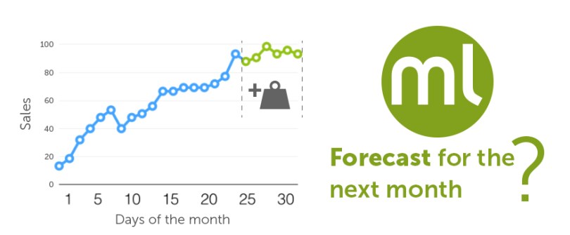
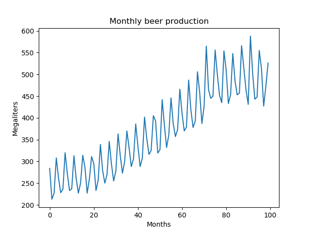
There are times when historical data inform certain behavior in the short or longer future. However, unlike the general classification or regression problems, Time Series needs your data to be organized as a sequence of snapshots of your input fields at various points in time. For example, the chart below depicts the variation of sales during a given month. Can we forecast the sales for future days or even months based on this data?

The answer is a resounding “Yes” since BigML has implemented the exponential smoothing algorithm to train Time Series models. In this type of models, the data is modeled as a combination of exponentially-weighted moving averages. Exponential smoothing is not new, it was proposed in the late 1950s. Some of the most relevant work was Robert Goodell Brown’s, in 1956, and later on, the field of study was expanded by Charles C. Holt in 1957, as well as Peter Winters in 1960. Contrary to other methods, in forecasts produced using exponential smoothing, past instances are not equally weighted and recent instances are given more weight than older instances. In other words, the more recent the observation the higher the associated weight.

From Zero to Time Series Forecasts

 

In BigML, a regular Time Series workflow is composed of training your data, evaluating it and forecasting what will happen in the future. In that way, it is very much like other modeling methods available in BigML. But what makes Time Series different?

1. The training data structure: The instances in the training data need to be sequentially arranged. That is, the first instance in your dataset will be the first data point in time and the last one will be the most recent one. In addition, the interval between consecutive instances must be constant.

2. The objective fields: Time Series models can only be applied to numeric fields, but a single Time Series model can produce forecasts for all the numeric fields in the dataset at once (as opposed to classification or regression models, which only allow one objective field per model). In other words, a Time Series model accepts multiple objective fields, and in fact you can use all numeric fields in the input dataset as objective at once.

3. The Time Series models. BigML automatically trains multiple models for you behind the scenes and lists them according to different criteria, which is a big boost in productivity as compared to hand tuning all the different combinations of the underlying configuration options. BigML’s exponential smoothing methodology models Time Series data as a combination of different components: level, trend, seasonality, and error (see Understanding Time Series Models section for more details).

When creating a Time Series, we have several options regarding whether to model each component additively or multiplicatively, or whether to include a component at all. To alleviate this burden, BigML computes in parallel a model for each applicable combination, allowing you to explore how your Time Series data fits within the entire family of exponential smoothing models. Naturally, we need some way to compare the individual models. BigML computes several different performance measures for each model, allowing you to select the model that best fits your data and gives the most accurate forecasts. Their parameters and corresponding formulas are described in depth in the Dashboard and API documentation.

4. Forecast: BigML lets you forecast the future values of multiple objective fields in short or long time horizons with a Time Series model. You will be able to separately train a different Time Series model for each objective field in just a few clicks. Your Time Series Forecasts come with forecast intervals: a range of values within which the forecast is contained with a 95% probability. Generally, these intervals grow as the forecast period increases, since there is more uncertainty when the predicted time horizon is further away.

5. Evaluation: Evaluations for Time Series models differ from supervised learning evaluations in that the training-test splits must be sequential. For an 80-20 split, the test set is the final 20% of rows in the dataset. Forecasts are then generated from the Time Series model with a horizon equal to the length of the test set. BigML computes the error between the test dataset values and forecast values and represents the evaluation performance in the form of several metrics: Mean Absolute Error (MAE), Mean Squared Error (MSE), R Squared, Symmetric Mean Absolute Percentage Error (sMAPE), Mean Absolute Scaled Error (MASE), and Mean Directional Accuracy (MDA). These metrics are fully covered in the Dashboard documentation.  Every exponential smoothing model type contained by a BigML Time Series model is automatically evaluated in parallel, so the end result is a comprehensive overview of all models’ performance.

Understanding Time Series Models

As mentioned in our description above, Time Series models are characterized by these four components:

• Level: Exponential smoothing, as the name suggests, reduces noisy variation in a Time Series’ value, resulting in a gentler, smoother curve. To understand how it works, let us first consider a simple moving average filter: for a given order m, the filtered value at time t is simply the arithmetic mean of the m preceding values, or in other words, an equally-weighted sum of the past m values. In exponential smoothing, the filtered value is a weighted sum of all the preceding values, with the weights being highest for the most recent values, and decreasing exponentially as we move towards the past. The rate of this decrease is controlled by a single smoothing coefficient α, where higher values mean the filter is more responsive to localized changes. In the following figure, we compare the results of filtering stock price data with moving average and exponential smoothing.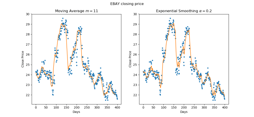Both smoothing techniques attenuate the sharp peaks found in the underlying Time Series data. The filtered values from exponential smoothing are what we call the level component of the Time Series model. Because the behavior of exponential smoothing is governed by a continuous parameter α, rather than an integer m, the number of possible solution is infinitely greater than the moving average filter, and it is possible to achieve a superior fit to the data by performing parameter optimization. Moreover, the exponential smoothing procedure for the level component may be analogously applied to the remaining Time Series components: trend and seasonality.
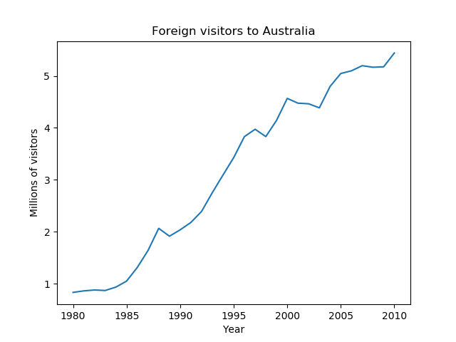
• Trend: While the level component represents the localized average value of a Time Series, the trend component of a Time Series represents the long term trajectory of its value. We represent trend as either the difference between consecutive level values (additive trend, linear trajectory), or the ratio between them (multiplicative trend, exponential trajectory). As with the level component, the sequence of local trend values is considered to be a noisy series which we can again smooth in an exponential fashion. The following series exhibits a pronounced additive (linear) trend.
• Seasonality: The seasonality component of a Time Series represents any variation in its value which follows a consistent pattern over consecutive, fixed-length intervals. For example, sales of alcohol may be consistently higher during summer months and lower during winter months year after year. This variation may be modeled as a relatively constant amount independent of the Time Series’ level (additive seasonality), or as a relatively constant proportion of the level (multiplicative seasonality). The following series is an example of multiplicative seasonality on a yearly cycle. Note that the magnitude of variation is larger when the level of the series is higher.
• Error: After accounting for the level, trend, and seasonality components. There remains some variation not yet accounted for by the model.  Like seasonality, error may be modeled as an additive process (independent of the series level), or multiplicative process (proportional to the series level). Parameterizing the error component is important for computing confidence bounds for Time Series Forecasts.

In Summary

To wrap up, BigML’s Time Series models:

• Help solve use cases such as predicting stock prices, sales forecasting, website traffic, production and inventory analysis as well as weather forecasting, among many other use cases.
• Are used to characterize the properties of ordered sequences, and to forecast their future behavior.
• Implement exponential smoothing, where the data is modeled as a combination of exponentially-weighted moving averages. That is, the recent instances are given more weight than older instances.
• Train the data with a different split compared to other modeling methods. The split needs to be sequential rather than random, so you can test your model against the latter period in your dataset.
• Are trained as level components and it can include other components such as: trend, damped, seasonality, or error.
• Let you forecast one or multiple objective fields. For multiple objectives, you can train a separate set of Time Series models for each objective field.

You can create Time Series models, interpret and evaluate them, as well as forecast short and longer horizons with them via the BigML Dashboard, our API and Bindings, plus WhizzML and Bindings (to automate your Time Series workflows). All of these options will be showcased in future blog posts.

Want to know more about Time Series?

At this point, you may be wondering how to apply Time Series to solve real-world problems. Rest assured, we’ll cover specific examples in the coming days. For starters, in our next post, we will show a use case where we will be examining a dataset with the number of houses sold in the United States since January 1963 to see if we can predict general or even seasonal trends. Stay tuned!

We hope this post made wet your appetite to learn more about Time Series. Please visit the dedicated release page for further learning. It includes a series of six blog posts about Time Series, the BigML Dashboard and API documentation, the webinar slideshow as well as the full webinar recording.