BigML’s Time Series Forecasting model uses Exponential Smoothing under hood. This blog post, the last one of our series of six about Time Series, will explore the technical details of Exponential Smoothing models, to help you gain insights about your forecasting results.
Exponential Smoothing Explained
To understand Exponential Smoothing, let’s first focus on the smoothing part of that term. Consider the following series, depicting the closing share price of EBAY over a 400 day period.
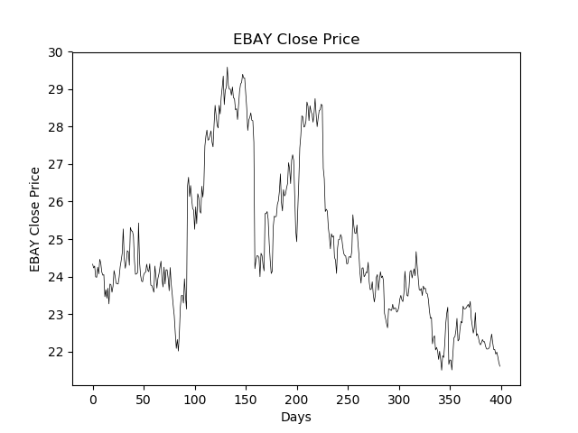
There is definitely some shape here, which can help us tell the story of this particular stock symbol. However, there are also quite a few transient fluctuations which are not necessarily of interest. One way to address this is to run a moving average filter over the data. 
The output of the moving average (MA) filter is shown as the blue line. At each time index, we compute the filtered data point as the arithmetic mean of the unfiltered data points located within a window of fixed width m about that time index. Given time series data y, a (symmetric) moving average filter produces the filtered series:

As seen in the figure, the resulting filtered time series contains only the large scale movements in the stock price, and so we have successfully smoothed the noise away from the signal.
When we apply Exponential Smoothing to a time series, we are performing an operation that is somewhat similar to the moving average filter. The exponential smoothing filter produces the following series:
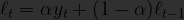
Where 


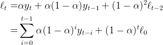
Where 

Why would we choose to smooth a time series using an exponential window instead of moving average? Conceptually, the exponential window is attractive because it allows the filter to emphasize a point’s immediate neighborhood without completely discarding the time series’ history. The fact that the parameter 
Now, the other half of time series modeling is creating forecasts. Both the moving average and exponential smoother have a flat forecast function. That is, for any horizon h beyond the final data point, the forecast is just the last smoothed value computed by the filter.

This is admittedly quite a simplistic result, but for stationary time series, these forecast values can be usable for reasonably short horizons. In order to forecast time series which exhibit more interesting movement, we need to incorporate trend into our model.
Trend models
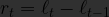
In the previous section we smoothed a time series using a single pass of an exponential window filter, resulting in a “level-only” model which produces flat forecasts. To introduce some motion into our exponential smoothing forecasts we can add a trend component to our model. We will define trend as the change between two consecutive level values 
- The difference between consecutive level values (additive trend):
- The ratio between consecutive level values (multiplicative trend):

We can then perform exponential smoothing on this trend value, in an identical fashion to the level value:

Where 

Hence, for additive trend models, the forecast is a straight line, and for multiplicative trend models, the forecast is an exponential curve. For some cases, it may be undesirable for the trend to continue at a constant value as the forecast horizon grows. We can introduce a damping coefficient 

and for multiplicative trend:

Seasonal models
Many time series exhibit seasonality, that is, a pattern of variation that takes over consecutive periods of fixed length. For example, alcohol sales may be higher during the summer than the winter, year after year, so a time series containing monthly sales figures of beer could exhibit a seasonal pattern with a period of m=12. Once again, seasonality can be modeled additively or multiplicatively. In the case of the former, the seasonal variation is independent of the level of series whereas in the latter, the variation is modeled as a proportion of the current level.
To bring it all together, the following is an example of a time series which exhibits both trend and seasonality.
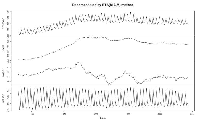
Note how the level is a smoothed version of the observed data, and the trend (labeled “slope”) is more or less the rate of change in the level.
Learning exponential smoothing models
Exponential smoothing models are fully specified by their smoothing coefficients α,β,γ , and φ along with initial state values l0, b0, and s0 (the remaining state values are obtained by running the smoothing equations forward). To evaluate how well an exponential smoothing model fits the data, we compute what is called the “within-sample one step ahead forecast error”. Put plainly, for each time step t, we compute the forecast for one step ahead, and calculate the error between the forecast and the actual data from the next time step.

We compute these errors for each time step where we have observed data available, and the sum of squared errors is our metric for model fit. This metric is then used to perform numeric optimization in order to obtain the best values for the smoothing coefficients and initial state values. BigML uses the Nelder-Mead simplex algorithm as its optimization solution.
Model Selection
Considering all the different combinations of trend and seasonality types for exponential smoothing can mean that we must choose among over a dozen different model configurations for a time series modeling task. Therefore, we need some way to rank the models against each other. Naturally, the ranking should incorporate a measure of how well the model fits the training time series, but should also help us avoid models which overfit the data. The tool that fits these requirements is the Akaike Information Criterion (AIC). Let 

Models which produce lower AIC values are considered better choices, so the best model is the one which maximizes the likelihood L, while minimizing the number of parameters k. Along with the AIC, BigML also computes two additional metrics for each model: the bias-corrected AIC (AICc), and the Bayesian Information Criterion (BIC). These quantities are still log-likelihood values penalized by model complexity. However the degree to which they punish extra parameters varies, with the BIC being most sensitive to the AIC being the least.
Want to know more about Time Series?
If you have any questions or you’d like to learn more about how Time Series work, please visit the dedicated release page. It includes a series of six blog posts about Time Series, the BigML Dashboard and API documentation, the webinar slideshow as well as the full webinar recording.
