BigML is bringing Time Series to the Dashboard to help you forecast future values based on your historical data. Time Series is widely used in forecasting stock prices, sales, website traffic, production and inventory levels among other use cases. This type of time-based data shows the common attribute of sequential distribution over time.

In this post, we will cover the six fundamental steps it takes to make forecasts by using Time Series in BigML, where you: upload your data, create datasets, train a Time Series model, analyze the results, evaluate your model and make forecasts.

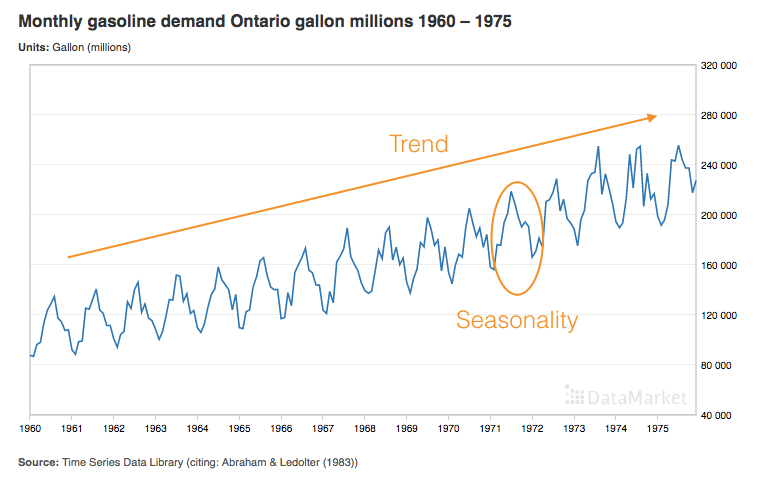
To illustrate each of these steps, we will use a dataset from DataMarket which contains the monthly gasoline demand in Ontario from 1960 until 1975. By looking at the chart below, we can observe two main patterns in the data: the seasonality  (more demand during summer vs. winter months) and an increasing trend over the years.

1. Upload your Data

Upload your data to your BigML account. BigML provides many options to do so, in this case, we drag and drop to the Dashboard the dataset we have previously downloaded from DataMarket.

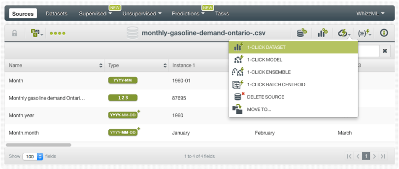
When you upload your data, the data type of each field in your dataset will be automatically detected by BigML. Time Series models will only use the numeric values in your dataset e.g., monthly gas demand field expressed in millions of gallons.

Important Note!

BigML indexes your instances in the same order they are arranged in the original source, i.e., the first instance (or row) is taken as the first data point in the series, the second instance is taken as the second data point and so on. Therefore you need to ensure that your instances are chronologically ordered in your source data.

2. Create a Dataset

From your Source view, in the 1-click action menu, use the 1-click Dataset option to create a dataset. This is a structured version of your data ready to be consumed by a Time Series.

Since Time Series is considered a supervised model you can evaluate it. You can use the 1-click split option to set aside some test data to later evaluate your model against. Since Time Series data is sequentially distributed, the split of the dataset needs to be linear instead of random. Using the configuration option shown in the image below, the first 80% instances of your dataset will be set aside for training and the last 20% for testing.

3. Create your Time Series

To train your Time Series you can either use the 1-click Time Series option or you can configure the parameters provided by BigML. BigML allows you to configure the following parameters:

• Objective fields: these are the fields you want to predict. You can select one or more objective fields and BigML will learn the Time Series models for each field separately, which further streamlines the training process.
• Default Numeric Value: if your objective fields contain missing values, you can easily replace them by the field mean, median, maximum, minimum or zero. By default, they are replaced by using spline interpolation.
• Forecast horizon: BigML presents a forecast along with your model creation so you can visualize it in the chart. The horizon is the number of data points that you want to forecast. You can always make a forecast for longer horizons once your model has been created.
• Model components: BigML models your data by exploring different variations of the error, trend and seasonality components. The combinations of these components result in the multiple models returned (see the introductory blog post of this series for a more detailed explanation):
  • Error: represents the unpredictable variations in the Time Series data, and how they influence observed values. It can be additive or multiplicative. Multiplicative error is only suitable for strictly positive data. By default, BigML explores all error variations.
  • Trend and damped: the trend component can be additive, generating a linear growth of the Time Series, or multiplicative, generating an exponential growth of the Time Series. Moreover, if a damped parameter is included, the trend of the Time Series will become a flat line at some point in the future. By default, BigML explores all trend variations.
  • Seasonality:  if your data contains fixed periods or fluctuations that occur in regular intervals, you need to include the seasonality component to your models. It can be additive or multiplicative, and the latter makes the seasonal variations proportional to the level of the series. By default, BigML explores both methods.
  • Period length: the number of data points per period in the seasonal data. The period needs to be set taking into account the time interval of your instances and the seasonal frequency. For example, for quarterly data and annual seasonality, the period should be 4, for daily data and weekly seasonality, the period should be 7.
• Dates: you can set dates for your data to visualize them afterward in the x-axis of the Time Series chart. BigML will calculate the dates for each instance by referencing the initial date associated with the first instance in your data and the row interval.

• Range: you may want to use a subset of instances to create your Time Series. This option is also handy if you haven’t yet split your dataset into training and tests sets.

In our example, we configure the seasonality component by selecting “All”, so BigML explores all possible seasonal combinations (additive and multiplicative) and a period length of 12 since we have monthly data and annual seasonality. We also select the initial date of our dataset with a row interval of 1 month because each of the instances represents a single month of data. At that point, we can simply click the Create button to form our Time Series.

4. Analyze your Results

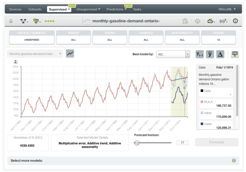
When your Time Series has been created you will see your field values and the best Time Series model plotted in a chart. As we mentioned before, BigML learns multiple models as a result of the different components combinations. The best model is selected taking into account the AIC (Akaike’s Information Criterion), but you can use any other of the metrics offered such as the AICc (Corrected Akaike’s Information Criterion), the BIC (Schwarz Bayesian Information Criterion) or the R squared. The preferred metric to select the best model is usually the AIC (or its variations, the AICc or the BIC) rather than the R squared, since it takes into account the trade-off between the model’s goodness-of-fit and the model’s complexity (to avoid overfitting) while the R squared only measures the degree of adjustment of the model to the data. The AICc is a variation of the AIC for small datasets and the BIC introduces a heavier penalization on model complexity.  To learn more about the model metrics read this article.

Below the chart, if you display the panel you will find a table containing all the different models learned from your data. You can visualize them by plotting them on the chart. Each model has a unique name which identifies its different components: Error, Trend, Seasonality. In our example, the model A,A,A is a model with Additive error, Additive trend, and Additive seasonality.

5. Evaluate your Time Series

You can evaluate a Time Series model using data that the model has not seen before. Just click on the Evaluate option in the 1-click action menu and BigML will automatically select the remaining 20% of the dataset that you set aside for testing.

When the evaluation has been created, you will be able to see your model plotted along with the test data data and the model forecasts. By default, BigML selects the best model by R squared measure, which quantifies the goodness-of-fit of the model to the test data and it can take values up to 1. You will also get different performance metrics for each of your models such as the MAE (Mean Absolute Error) and the MSE (Mean Squared Error). The lower the MAE and the MSE and the higher the R squared the better. You can see below that our model has a very good performance on the test data with an R squared of 0.9833.

The table within the panel below displays all the related models and other metrics such as sMAPE (symmetric Mean Absolute Percentage Error), which is similar to the MAE except the model errors are measured in percentage terms, the MASE (Mean Absolute Scaled Error) and the MDA (Mean Directional Accuracy), which compares the forecast direction (upward or downward) to the actual data direction. See this article for detailed explanations.

6. Make Forecasts

From your model view, you will be able to see the forecasts of your selected models with up to 50 future data points. If you want to predict a longer horizon, you can click on the option to extend it. You can also compare your model forecast with three other benchmark models: a model that always predicts the mean, a naive model that always predicts the last value of the series and a drift model that draws a straight line between the first and last observation of the series and extrapolates the future values.

Want to know more about Time Series?

Please visit the dedicated release page for further learning. It includes a series of six blog posts about Time Series, the BigML Dashboard and API documentation, the webinar slideshow as well as the full webinar recording.