At BigML we’re well aware that data preparation and feature engineering are key steps for the success of any Machine Learning project. A myriad of splendid tools can be used for the data massaging needed before modeling. However, in order to simplify the iterative process that leads from the available original data to a ML-ready dataset, our platform has recently added more data transformation capabilities. By using SQL statements, you can now aggregate, remove duplicates, join and merge your existing fields to create new features. Combining these new abilities with Flatline, the existing transformation language, and the platform’s out-of-the-box automation and scalability will help greatly to solve any real Machine Learning problem.

The data: San Francisco Restaurants

Some time ago we wrote a post describing the kind of transformations needed to go from a bunch of CSV files that contained information about the inspections of some restaurants and food businesses in San Francisco. The data was published by the San Francisco’s Department of Public Health and was structured in four different files:

• businesses.csv: a list of restaurants or businesses in the city.
• inspections.csv: inspections in some of previous businesses.
• violations.csv: detected law violations in some of previous inspections.
• ScoreLegend.csv: a legend to describe score ranges.

The post described how to build a dataset that could be used to do Machine Learning with them using MySQL. Let’s compare now how could you do that using BigML’s newly added transformations.

Uploading the data

As explained in the post, the first thing that you need to do to use this data in MySQL is defining the structure of the tables where you will upload it, so you need to care about the contents of each column and assign the correct type after a detailed inspection of each CSV file. This means writing commands like this one for every CSV.

create table business_imp (business_id int, name varchar(1000), address varchar(1000), city varchar(1000), state varchar(100), postal_code varchar(100), latitude varchar(100), longitude varchar(100), phone_number varchar(100));

and some more to upload the data to the tables:

load data local infile '~/SF_Restaurants/businesses.csv' into table business_imp fields terminated by ',' enclosed by '"' lines terminated by '\n' ignore 1 lines (business_id,name,address,city,state,postal_code,latitude,longitude,phone_number);

and creating indexes to be able to do queries efficiently:

create index inx_inspections_businessid on inspections_imp (business_id);

The equivalent in BigML would be just drag and dropping the CSVs in your Dashboard:

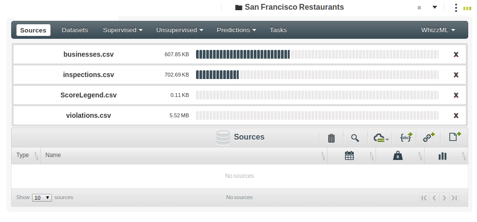And as a result, BigML infers for you the types associated to every column detected in each file. In addition, the types being assigned are totally focused on the way the information will be treated by the Machine Learning algorithms. Thus, in the inspections table we see that the Score will be treated as a number, the type as a category and the date is actually automatically separated into the year, month and day components, which are the ones meaningful in the ML processes.

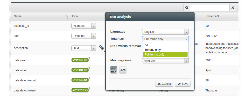
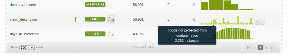
We just need to verify the inferred types in case we want some data to be interpreted differently. For instance, the violations file contains a description text that includes information about the date the violation was corrected.

$ head -3 violations.csv
"business_id","date","description"
10,"20121114","Unclean or degraded floors walls or ceilings [ date violation corrected: ]"
10,"20120403","Unclean or degraded floors walls or ceilings [ date violation corrected: 9/20/2012 ]"

Depending on how you want to analyze this information, you can decide to leave it as it is, and contents will be parsed to produce a bag of words analysis, or set the text analysis properties differently and work with the full contents of the field.

As you see, so far BigML has taken care of most of the work, defining the fields in every file, their names, the types of information they contain, parsing datetimes and text. The only remaining contribution we think of now is taking care of the description field, which in this case combines information about two meaningful features: the real description and the date when the violation was corrected.

Now that the data dictionary has been checked, we can just create one dataset per source by using the 1-click dataset action.

Transforming the description data

The same transformations described in the above-mentioned post can be applied now from using the BigML Dashboard. The first one is removing the [date violation corrected: …] substring from the violation’s description field. In fact, we can go further and use that string to create a new feature: the days it took for the violation to be corrected.

This kind of transformations was already available in BigML thanks to Flatline, our domain-specific transformation language.

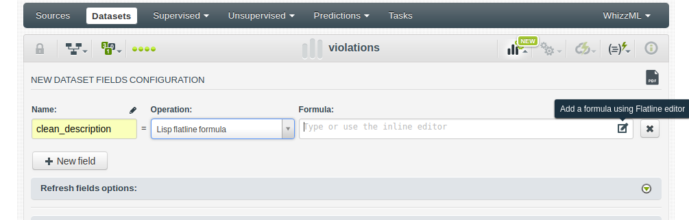
Using a regular expression, we can create a clean_description field removing the date violation part

(replace (f "description")
            "\\[ date violation corrected:.*?\\]"
            "")

Previewing the results of any transformation we define is easier than ever thanks to our improved Flatline Editor.

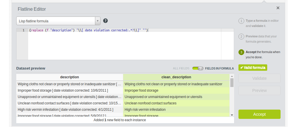
By doing so, we discover that the new clean_description field is assigned a categorical type because its contents are not free text but a limited range of categories.

The second field is computed using the datetime capabilities of Flatline. The expression to compute the days that took to correct the violation is:

(/ (- (epoch (replace (f "description")
                      ".*\\[ date violation corrected: (.*?) \\]"
                      "$1") "MM/dd/YYYY")
      (epoch (f "date") "YYYYMMdd"))
   (* 1000 24 60 60))

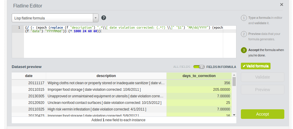
where we parsed the date in the original description field and subtracted the one that the violation was registered in. The difference is stored in the  days_to_correction new feature, to be used in the learning process.

Getting the ML-ready format

We’ve been working on a particular field of the violations table so far, but if we are to use that table to solve any Machine Learning problem that predicts some property about these businesses, we need to join all the available information in a single dataset. That’s where BigML‘s new capabilities come handy, as we now offer joins, aggregations, merging and duplicate removal operations.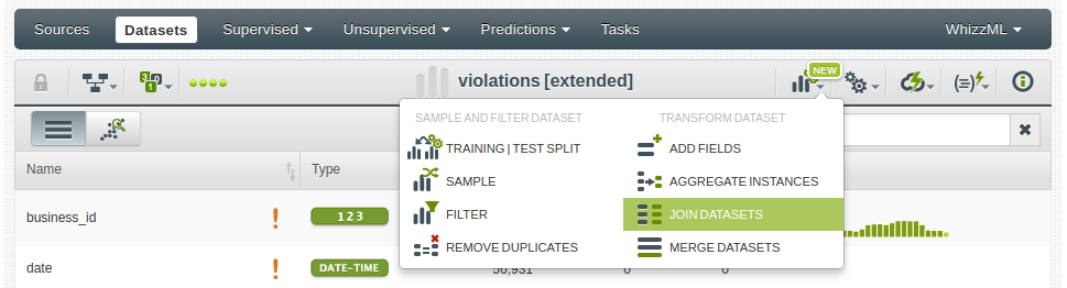                       

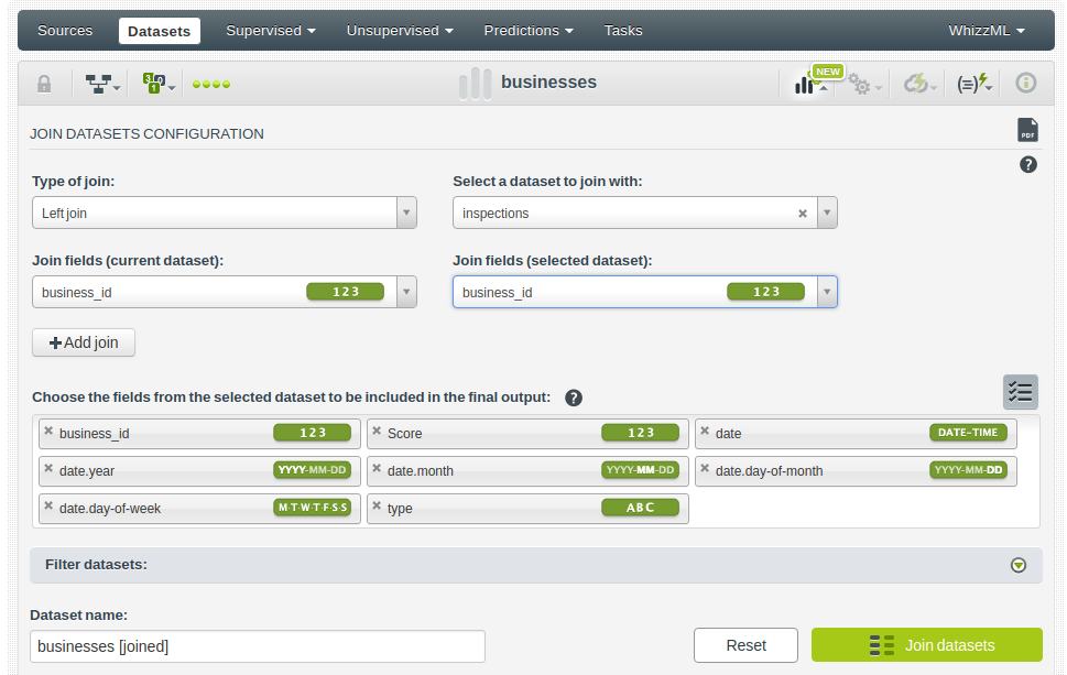
In this case, we need to join the businesses table with the rest, and we realize that inspections and violations use the business_id field as the primary key, so a regular join is possible. The join will keep all businesses and every business can have none or multiple related rows in the other two tables. Let’s join businesses and inspections:

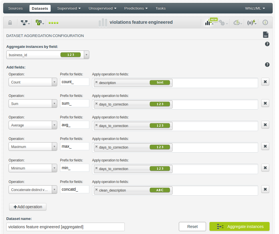
Now, to have a real ML-ready dataset, we still need to meet a requirement. Our dataset needs to have a single row for every item we want to analyze. In this case, it means that we need to have a single row per business. However, joining the tables has created multiple rows, one per inspection. We’ll need to apply some aggregation: counting inspections, averaging scores, etc.

The same should be done for the violations table, where again each business can have multiple violations. For instance, we can aggregate the days that it took to correct the violations and the types of violation per business.

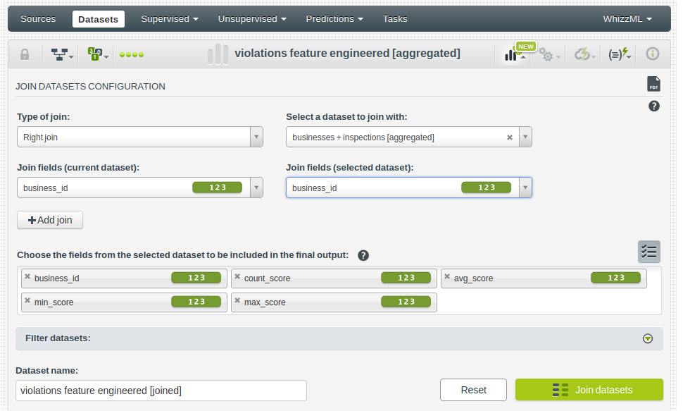
And now, use a right join to add this information to every business record.

Finally, the ScoreLegend table is just providing a list of categories that can be used to discretize the scores into sensible ranges. We can easily add that to the existing table with a simple select * from A, B expression plus a filter to select the rows whose Score field value is between the Minimum_Score and Maximum_Score of each legend. In this case, we’ll use the more full-fledged API capabilities through the Python bindings.

# applying the sql query to the business + inspections + violations
# dataset and the ScoreLegend
from bigml.api import BigML
api = BigML()
legend_dataset = api.create_dataset( \
    [business_ml_ready,
     score_legend],
    {"origin_dataset_names": {
        business_ml_ready: "A",
        score_legend: "B"},
     "sql_query": "select * from A, B"})
api.ok(legend_dataset)

# filtering the rows where the score matches the corresponding legend
ml_dataset = api.create_dataset(\
    legend_dataset,
    {"lisp_filter": "(<= (f \"Minimum_Score\")" \
                    " (f \"avg_score\")" \
                    " (f \"Maximum_Score\"))"})

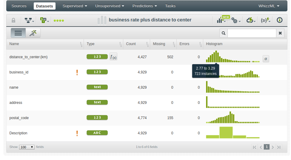
With these transformations, the final dataset is eventually Machine Learning ready and can be used to cluster restaurants in similar groups, find out the anomalous restaurants, or classify them according to their average score ranges. Nevertheless, we can generate new features, like the distance to the city center, or the rate of violations per inspection. These transformations can help to better describe the patterns in data. Here’s the Flatline expression needed to compute the distance of the restaurants to the center of San Francisco using the Haversine formula.

(let (pi 3.141592
      lon_sf (/ (* -122.431297 pi) 180)
      lat_sf (/ (* 37.773972 pi) 180)
      lon (/ (* (f "longitude") pi) 180)
      lat (/ (* (f "latitude") pi) 180)
      dlon (- lon lon_sf)
      dlat (- lat lat_sf)
      a (+ (pow (sin (/ dlat 2.0)) 2) (* (cos lat_sf) (cos lat) (pow (sin (/ dlon 2.0)) 2)))
      c (* 2 (/ (sqrt a) (sqrt (- 1 a)))))
 (* 6373 c))

For instance, modeling rating in terms of the name, address, postal code or distance to the city center could give us information about how to look up for the best restaurants.

Trying a logistic regression, we learn that to find a good restaurant, it’s best to move a bit away from the center of San Francisco.

Having data transformations in the platform has many advantages. Feature engineering becomes an integrated feature, so trivial to be used, and scalability, automation and reproducibility are granted, as for any other resource (and one click away thanks to Scriptify). So don’t be shy and give it a try!