The BigML Team has been working hard to bring OptiML to the platform, which will be available on May 16, 2018. As explained in our previous post, OptiML is an automatic optimization process for model selection and parametrization (or hyper-parametrization) to solve classification and regression problems. Selecting the right algorithm and its optimum parameter values is a manual and time-consuming task for any Machine Learning practitioner. This iterative process is currently based on trial and error (creating and evaluating different models to find the best one) and it requires a high level of expertise and intuition. OptiML accelerates the process of model search and parameter tuning, allowing non-experts to build top-performing models.

In this post, we will take you through the four necessary steps to find the top-performing model for your data using OptiML with the BigML Dashboard. We will use the Loan risk dataset which contains data from loan applicants to predict if whether applicants will be good or bad loan customers.

1. Upload your Data

As usual, you need to start by uploading your data to your BigML account. BigML offers several ways to do so: you can drag and drop a local file, connect BigML to your cloud repository (e.g., S3 buckets), or copy and paste a URL. This will create a source in BigML.

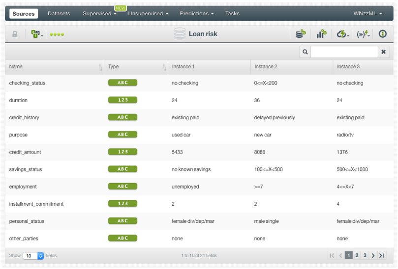
BigML automatically identifies the field types. In this case, we have 21 different fields. You can observe in the image below an excerpt of the fields for this loan risk dataset, such as the checking status, duration of the applied loan, credit history of the applicant and more.

2. Create a Dataset

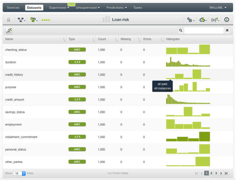
From your source view, use the 1-click dataset menu option to create a dataset, a structured version of your data ready to be consumed by a Machine Learning algorithm.

When your dataset is created, you will be able to see a summary of your field values, some basic statistics, and the field histograms to analyze your data distributions. You can see that our dataset has a total of 1,000 instances. Our objective field is the “class”, a categorical field containing two different classes that label loan customers as “good” (700 instances) or “bad” (300 instances).

3. Create an OptiML

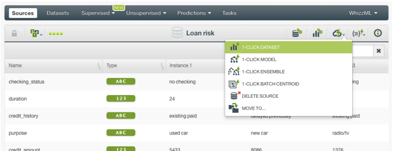
In BigML, you can use the 1-click OptiML menu option (shown on the left in the image below), which will use the default parameter values, or you can manually tune the parameters using the Configure OptiML option (shown on the right in the image below).

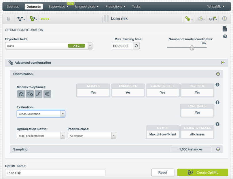
BigML allows you to configure the following parameters for your OptiML:

• Maximum training time: an upper bound to limit the OptiML runtime. If all the model candidates are trained faster than the maximum time set, the OptiML will finish earlier. By default, it is set to 30 minutes. However, for big datasets, this may be too short and you will need to set a longer time for the OptiML to build and evaluate more models.
• Model candidates: the maximum number of different models (i.e. models using a unique configuration) to be trained and evaluated during the OptiML process. The default is 128 which is usually enough to find the best model, but you can set it up to 200. The top-performing half of the model candidates will be returned in the final result.
• Models to optimize: the algorithms that you want to be optimized: decision trees, ensembles (including Boosted trees and Random Decision Forests), logistic regressions (only for classification problems), and deepnets. By default, all types of models are optimized.
• Evaluation: the strategy to evaluate the models and select the top performing ones. By default, BigML performs Monte Carlo cross-validation. Cross-validation evaluations usually yield more accurate results than single evaluations since they avoid the potential error derived from randomly selecting a too optimistic test dataset. Alternatively, you can select a specific test dataset if you need to optimize your models that way. To avoid unrealistically high performing evaluations due to the lack of cross-validation, BigML takes several subsets of the training data to build the same models and evaluates them using the test dataset.
• Optimization metric and the Positive class: the optimization metric is used for model selection during the optimization process. For regression problems, BigML uses the R squared by default and the maximum phi coefficient for classification problems. However, you can also select other metrics such as the accuracy, the ROC AUC, or the F measure. (All these metrics are explained in detail in the evaluations chapter of the BigML Dashboard documentation.) For classification problems, you can also select a positive class to be optimized; otherwise, the average metric for all classes will be optimized.
• Sampling: you can specify a subset of the instances of your dataset to create the OptiML.

Analyze the OptiML Results

While your OptiML is being created, you will be able to observe a set of metrics to track the progress. Apart from the typical progress bar that you can find for all BigML resources, you can also see the elapsed time (which should not be higher than the maximum training  time configured), the number of models evaluated, the total resources created (taking into account models, datasets and evaluations), the total data size processed, and the scores of the last models evaluated.

Once your OptiML is created, you can visualize the results in the OptiML view which is mainly composed of a chart and a table. This view allows you to compare and select the models that better suit your needs.

By looking at the chart, you can see the models ranked (from left to right) by the optimization metric score. If you mouse over the bars as shown in the image below, you will be able to see the model score +/- the standard deviation (calculated by using the different evaluations from the cross-validation) and the relevant model characteristics. Clicking on each bar, redirects you to the individual model view.

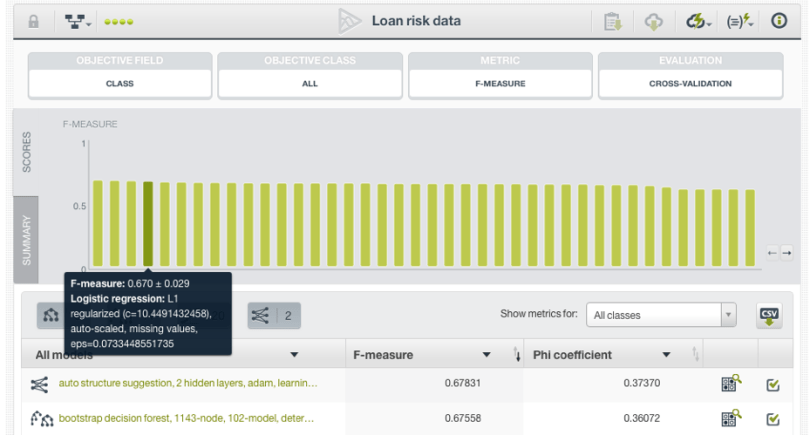
We can see below that this OptiML execution selected 8 decision trees, 11 ensembles, 20 logistic regressions, and 2 deepnets as the best models. In this case, the top-performing model is a deepnet with an f-measure of 0.67832, but the difference in performance in comparison with the following ensemble (with an f-measure of 0.67558) is not significant. If you look at the standard deviation, which indicates the potential variation of the f-measure depending on the random split of the dataset to train and evaluate the model, it is 0.02569 for out top model. This means that the f-measure for this model can take values from (0.67832-0.02569) = 0.65263 to (0.67832+0.02569) = 0.70401. Therefore, in this case you may prefer to select the second or third models in the list which are ensembles rather than a deepnet because they are easier to interpret and they are fatser to train.

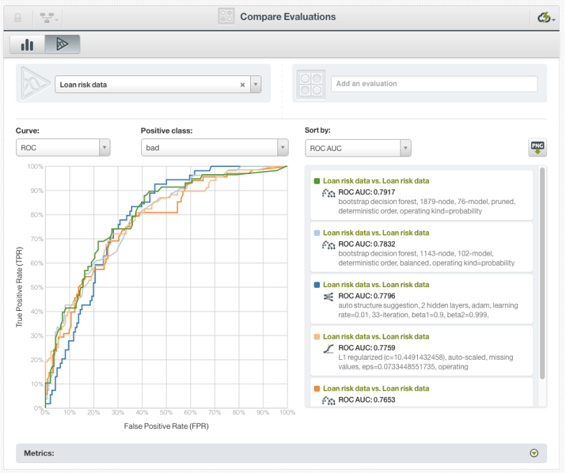
You can select multiple models from the table (up to 20 for classification) and click the button “Compare evaluations” (see above) to compare them in the BigML evaluation comparison chart (see below). The ROC curve along with other evaluation measures (precision-recall, gain and lift curves) are also plotted in a chart so you can easily make comparisons and settle on the model of your choice.

Each of the OptiML models can be found in your Dashboard listings under the OptiML tab as seen below. This is important to keep your Dashboard organized and to prevent mixing dozens of automatically created models with your manually configured models outside of OptiML. Keep in mind that the evaluations and the datasets created during the cross-validation phase are not listed in the Dashboard, but you can easily access them from the OptiML view.

4. Making Predictions from your Models

Comparing and analyzing several models helps you decide which is the best model for your particular use case. Once you have selected the model, you can start making predictions with it.

Single predictions

To make predictions for a single instance, simply click on the Predict option from the OptiML view (see below) or from the model view.

A form containing all your input fields will be displayed and you will be able to set the values for a new instance. At the top of the view, you will also get all the objective class probabilities for each prediction. Remember that you can always ask for the prediction explanation, a feature recently added to BigML that provides more context and transparency to the underlying logic of the selected algorithm as applicable to a given prediction.

Batch predictions

If you want to make predictions for multiple instances at the same time, click on the Batch Prediction option and select the dataset containing the instances for which you want to know the objective field value.

You can configure several parameters for your batch prediction such as the option to include all class probabilities in the output dataset and file. When your batch prediction finishes, you will be able to download the CSV file and view the output dataset.

Want to know more about OptiML?

If you have any questions or you would like to learn more about how OptiML works, please visit the release page. It includes a series of blog posts, the BigML Dashboard and API documentation, the webinar slideshow as well as the full webinar recording.