The BigML Team is bringing operating thresholds for your classification model evaluations and predictions. As explained in our previous posts, operating thresholds are a way to improve the performance of your models, especially when the objective field contains an imbalanced distribution for your classes.

Operating thresholds are only meant to be used for classification problems, i.e., the objective field must be categorical. For these problems, a Machine Learning algorithm is used to build a model that predicts a category. The objective field can have two or more categories, for example, “true or false”, “fraud or not fraud”, “high risk, low risk or medium risk”, etc. In these type of problems, there is always one class more important than the others (e.g., “fraud” or “high risk” are more important than “no fraud”, or “low risk”). Operating thresholds allow you to improve the performance of your class of interest. In our previous post we presented a case study that showcased how to reduce False Negatives with operating thresholds. In this post, you’ll learn how to use operating thresholds for classification models step by step in the BigML Dashboard.

1. Upload your Data

As usual, you need to start by uploading your data to your BigML account. This will create a source in BigML.

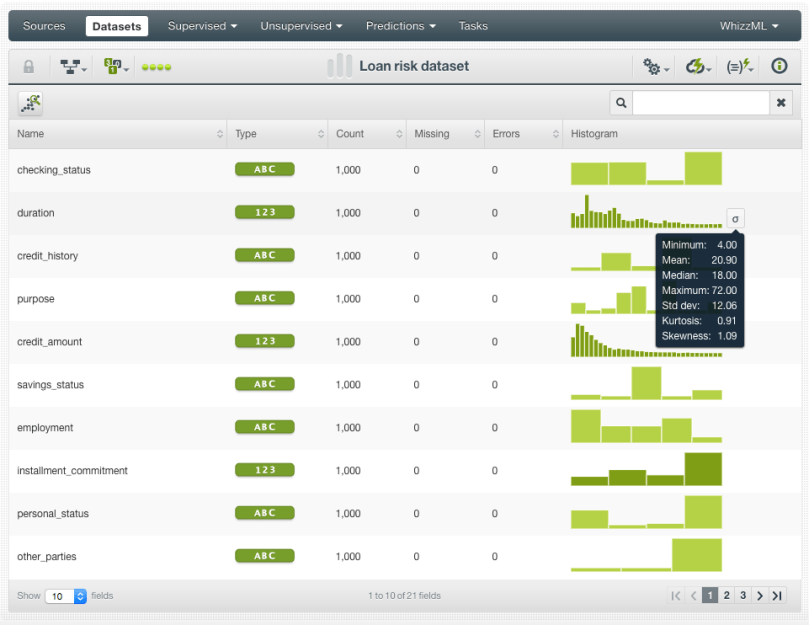
For illustrating purposes, we select a dataset containing different loans and the goal is to predict the risk per loan: “good” means the loan is not risky, “bad” means the loan is risky. You can see in the image below the different variables we have for each loan such as the duration of the loan or the credit amount.

2. Create a Dataset

From your source view, use the 1-click dataset menu option to create a dataset. In the dataset view, you will be able to see a summary of your field values and some basic statistics. You can see that our dataset has a total of 1,000 instances with no missing values and no errors.

For the objective field, we have 700 instances of the “good” class and 300 instances of the “bad” class. This is an example of an imbalanced dataset in Machine Learning since we have a significantly different number of instances for each of our objective field classes. This difference will likely bias the model to predict the majority class at the expense of the minority class since this is the way for the model to maximize performance. The problem is that the minority class is usually our class of interest as in this case, where we are more interested in predicting the risky loans than the not risky ones.

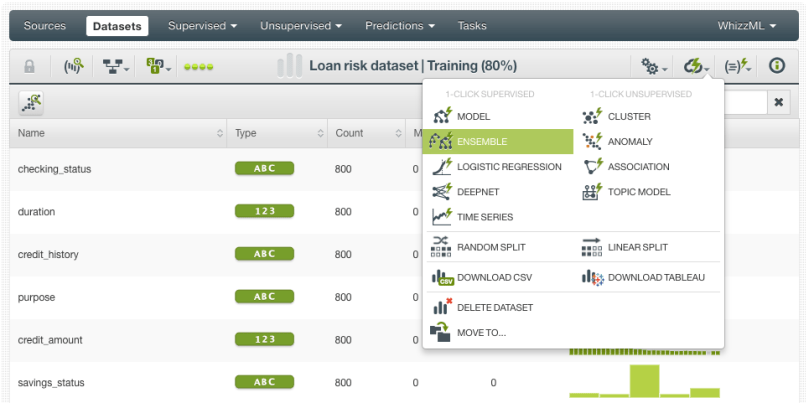
Before building the model, we are randomly splitting our dataset into two subsets: 80% for training and 20% for evaluating to ensure that the model generalizes well against unseen data. You can easily do this by using the BigML option under the 1-click action menu.

3. Create a Classification Model

BigML provides different algorithms that you can use to build a classification model: decision trees, ensembles, logistic regressions, and deepnets (Deep Neural Networks). In this case, we are building an ensemble using the 80% of the dataset with the 1-click option which uses default values for the ensemble parameters. By default, BigML takes the last field in the dataset as the objective field.

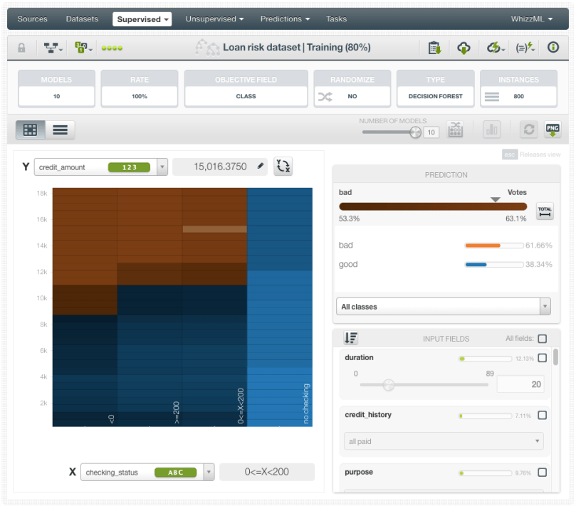
When your ensemble is created, you can visualize it in a Partial Dependence Plot (PDP), to analyze the marginal impact of the selected fields on the objective field predictions.

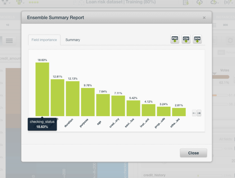
You can also see the top predictors by clicking on the summary report, available on the top menu. In this case, you can observe that the most important fields to predict the delinquency risk are the checking status, the loan amount, and the loan duration.

4. Evaluate your Classification Model

When your model is created, you need to evaluate it to ensure it is performing satisfactorily against new data instances. We use the 20% of the dataset that we set aside for the evaluation. You can see the results of the model evaluation below.

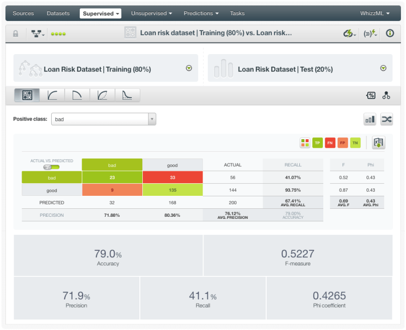
Although we got an acceptable overall performance (79% of accuracy) for our simple 1-click model, you can see that the “good” class has a better performance than the “bad” class. The model is predicting right 135 out of 144 instances of the “bad” class (~94% of recall), compared to the 23 right out of 33 instances (~41% of recall) for the good class. Also, the precision turns out better for the “good” class (~80% versus 72% precision). The model is clearly prioritizing the “good” class because it is the majority class. However, our positive class, i.e., our class of interest, is the “bad” class since our main goal is to stop losing money giving away loans that are susceptible to defaults.

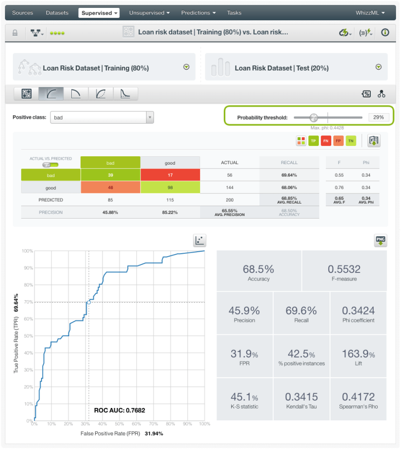
To improve the performance of our positive class, we can set an operating threshold. In this case, we will set a threshold based on the class probability, but you can also set it based on the confidence or votes (for ensembles) by configuring the prediction (as explained in the predictions section). By setting a probability threshold you are establishing the following criteria for the model: if the positive class probability is greater than the established threshold, then the positive class will be predicted, otherwise, the following class with the highest probability will be predicted. You can observe the total predictions and the recall for the positive class increasing as we lower our threshold. By setting a 29% of threshold we have 85 instances predicted as the “good” class and a ~70% of recall compared to the 32 instances and the ~41% of recall without setting a threshold.

If we set a 20% threshold instead, the recall increases up to ~88%. As usual, there is no free lunch. The downside of increasing the recall is the decrease in precision. From the ~72% of precision that we had without thresholds down to the ~45% precision for a 20% threshold.

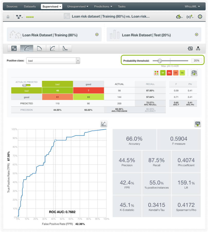
However, the precision is usually less important than the recall for most classification problems. In our example, predicting a loan that will be “good” as “bad” (false positive), is not as costly as predicting a loan that will be “bad” as “good” (false negative). For example, imagine that we establishing stricter conditions for “bad” loan applications than for “good” ones. Predicting a loan that will be “good” as “bad” may result in losing some customers that would be good customers as they don’t meet our strict conditions.  This loss has an opportunity cost associated, but it is likely lower than the cost of giving away a loan that will not be repaid or that will take a long time and effort to get paid back.

The key decision during the model’s evaluation is the optimal threshold to make predictions by taking into account the different costs of false negatives and false positives.

5. Make Predictions Using an Operating Threshold

Once you evaluate your model and decide the optimal threshold, you can start making predictions with it by using brand new instances. BigML allows you to set thresholds for both single and batch predictions.

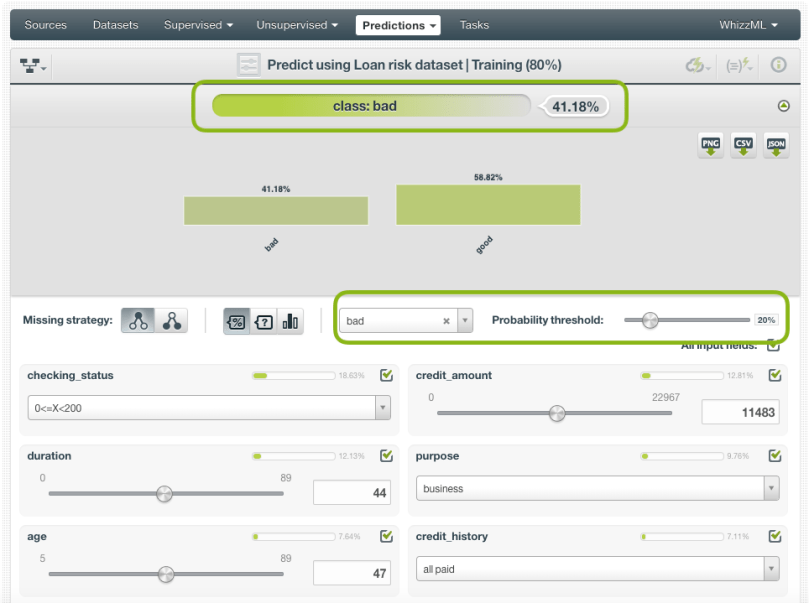
For single predictions, you will get the prediction on top and the histogram of the class probabilities distribution below. In the image below, you can see that given the input data, the prediction is “good” with 59% of probability.

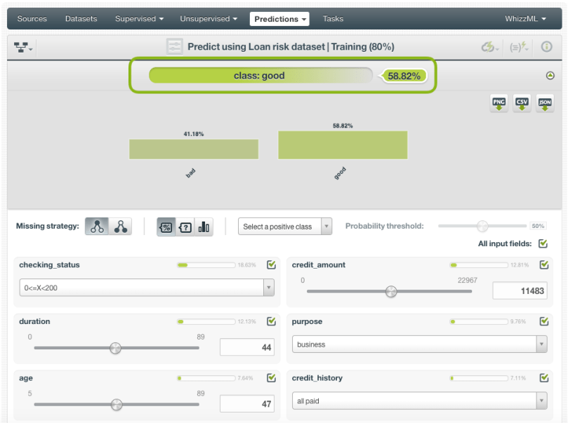
If we decided that the optimal threshold should be 20% for the “bad” class, it will be predicted only when its probability is greater than 20%. You can see how the prediction changes by setting a probability threshold.

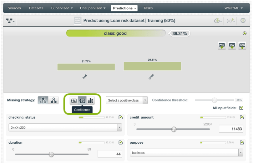
For non-boosted ensembles, apart from the probability, you can also select a threshold based on the confidence or the votes of the classes. The confidence is a pessimistic measure of the class probability, while the votes represent the percentage of trees voting for a given class in the ensemble.

For batch predictions, you can also select the strategy (probability, confidence or votes) and the threshold to use in the prediction from the configuration panel as shown in the image below.

Want to know more about operating thresholds?

If you have any questions or you’d like to learn more about how operating thresholds work, please visit the dedicated release page. It includes a series of six blog posts about operating thresholds, the BigML Dashboard and API documentation, the webinar slideshow as well as the full webinar recording.