So far, as presented in our introductory blog post, we have learned about what operating thresholds are and how they can be useful. Now it is time to deal with an actual dataset and see how altering operating thresholds can improve the predictions of your real world problems. Many datasets in the real world are unbalanced, with a large difference between the population of the objective classes. Moreover, often times a minority class is very important to detect (fraud detection, loan risk, medical screening, etc.) If we consider a minority class to be the positive class, we may want to keep false negatives (i.e., missed detections) as low as possible. There is no free lunch, but we can always choose to lower the false negatives at the cost of increasing our false positives. This is important if we want to make sure we don’t miss out detecting our rare class.

The Dataset

Once such dataset is customer churn in the telecom industry. As sample churn dataset can be found in the BigML Gallery among public datasets. It has many fields, both numeric and categorical, that might correlate to churn in some way, but the objective field is binary — did the account get canceled or not. This dataset is imbalanced since only about 17% of the instances are “True”, when the customer ended their service.

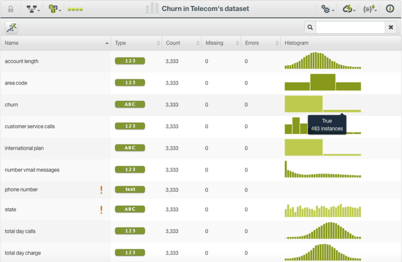
Although canceling an account does not happen frequently, it is very important to detect in this context. In particular, we really want to know ahead of time if an account is likely to be canceled. It costs very little to send an apology email or make a free offer compared to losing repeat business, so it is better to send such an email when necessary versus doing nothing and losing a customer.

The Model

After cloning our dataset from the gallery, we proceed with the traditional Machine Learning workflow by splitting the dataset into a test and training set. Then, we create a Bagging ensemble with 30 models on the training set. At this point, we can evaluate this ensemble against the test set as follows.

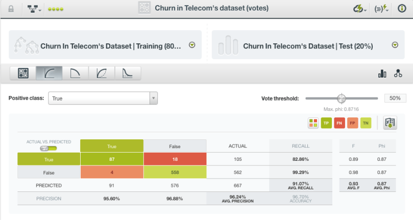
Let’s check out the ROC view and set the positive class to “True”, meaning that we predict that the customer will churn. Looking at the confusion matrix, we can see there are 21 false negatives. To the right, we have the ability to set the probability threshold with a simple slider. The probability threshold corresponding to the maximum phi is already marked. This is a way of maximizing the trade-off between precision and recall in a way that balances false positives and false negatives. This, however, is also assuming that either type of mistake is equally bad.

However, our scenario is different. We don’t want a balance between false positives and false negatives; false negatives are costly to us and we want to minimize them at the expense of more false positives. In this case, we can pull the slider even further down, say to 10%. This decreases our false negatives by about a third but increases our false positives ten-fold! Depending on how costly these kinds of mistakes are, this may still be a worthwhile trade-off. So, where is the optimum threshold? It depends on the costs associated with your particular problem.

Since we have used an ensemble, we can also influence which customers are predicted to churn by changing the underlying voting strategy. The voting strategy determines how the 30 different predictions from our 30 different models are combined to make a final prediction. We can choose between probability (which averages the per-class probability from each model), confidence (which average the per-class confidence), and voting (which simply gives each model a single vote).

Let’s go back to our ensemble and click to create a new evaluation. This time, we click on the dropdown for Configure options. We can now choose how we want our predictions combined. 

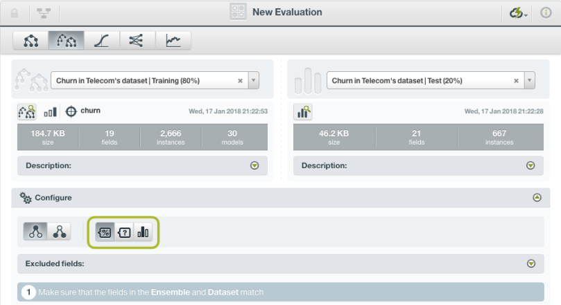
As we try different options, for this ensemble, we observe that there isn’t a significant difference between the different methods. (The false negatives and average precision are very similar, as shown in the two images below.)

Don’t let this example fool you though. In general, confidences are a pessimistic approach to measuring certainty in a prediction, and they can vary significantly from probabilities when there are only a few instances in a decision tree’s leaf node. We can explore this in the new version of BigML model view. Click on the first model in our ensemble to view it. To the right, you will now have the choice of viewing by probability or by confidence. For example, here is a node with only four points in it, and they are all false.

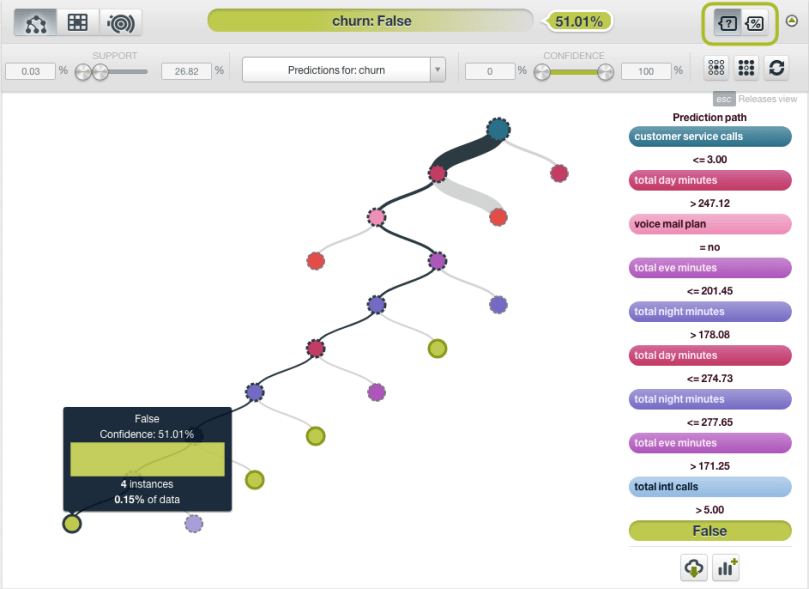
The probability of a point at this node being false is quite high since all the current points are false, yet there are so few such instances that it is hard to make this claim with much confidence. So, it is no surprise that the confidence value is much lower.  

This has been a quick walkthrough of what changing operating thresholds might look like with a real dataset. We can easily alter the number of false positives and false negatives tolerated by adjusting the probability threshold, though it takes domain-specific knowledge to determine exactly where the optimum threshold should be. Provided that you have in-depth knowledge of your data, you can tailor the predictions to your needs and greatly improve the performance of your model.

Want to know more about operating thresholds?

If you have any questions or you’d like to learn more about how operating thresholds work, please visit the dedicated release page. It includes a series of six blog posts about operating thresholds, the BigML Dashboard and API documentation, the webinar slideshow as well as the full webinar recording.