Over our last few blog posts, we’ve gone through the various ways you can use BigML’s new Deepnet resource, via the Dashboard, programmatically, and via download on your local machine. But what’s going on behind the curtain? Is there a little wizard pulling an elaborate console with cartoonish-looking levers and dials?

Well, as we’ll see, Deepnets certainly do have a lot of levers and dials.  So many, in fact, that using them can be pretty intimidating. Thankfully, BigML is here to be your wizard* so you aren’t the one looked shamefacedly at Dorothy when she realizes you’re not as all-powerful as you might have thought.

Deepnets:  Why Now?

First, let’s address an important question, why are deep neural networks suddenly all the rage?  After all, the Machine Learning techniques underpinning deep learning have been around for quite some time. The reason boils down to a combination of innovations in the technology supporting the learning algorithms more than advances in learning algorithms themselves. It’s worth quoting Stuart Russell at length here:

. . .deep learning has existed in the neural network community for over 20 years. Recent advances are driven by some relatively minor improvements in algorithms and models and by the availability of large data sets and much more powerful collections of computers.

He gets at most of the reasons in this short paragraph.  Certainly, the field has been helped along by the availability of huge datasets like the ones generated by Google and Facebook, as well as some academic advances in algorithms and models.

But the things I will focus on in this post are in the family of “much more powerful collections of computers”.  In the context of Machine Learning, I think this means two things:

• Highly parallel, memory-rich computers provisionable on-demand.  Few people can justify building a massive GPU-based server to train a deep neural network on huge data if they’re only going to use it every now and then. But most people can afford the same for a few days at a time. Making such power available in this way makes deep learning cost-effective for far more people than it used to be.
• Software frameworks that have automatic differentiation as first-class functionality. Modern computational frameworks (like TensorFlow, for example) allow programmers to instantiate a network structure programmatically and then just say “now do gradient descent!” without ever having to do any calculus or worry about third-party optimization libraries.  Because differentiation of the parameters with respect to the input data is done automatically, it becomes much easier to try a wide variety of structures on a given dataset.

The problem here then becomes one of expertise:  people need powerful computers to do Machine Learning, but few people know how to provision and deploy machines on, say Amazon AWS to do this. Similarly, computational frameworks to specify and train almost any deep network exist and are very nice, but exactly how to use those frameworks and exactly what sort of network to create are problems that require knowledge in a variety of different domains.

Of course, this is where we come in. BigML has positioned itself at the intersection of these two innovations, utilizing a framework for network construction that allows us to train a wide variety of network structures for a given dataset, using the vast amount of available compute power to do it quickly and at scale, as we do with everything else. We add to these innovations a few of our own, in an attempt to make Deepnet learning as “hands off” and as “high quality” as we can manage.

What BigML Deepnets are (currently) Not:

Before we get into exactly what BigML’s Deepnets are let’s talk a little bit about what they aren’t. Many people who are technically minded will immediately bring to mind the convolutional networks that do so well on vision problems, or the recurrent networks (such as LSTM networks) that have great performance on speech recognition and NLP problems.

We don’t yet support these network types.  The main reason for this is that these networks are designed to solve supervised learning problems that have a particular structure, not the general supervised learning problem.  It’s very possible we’ll support particular problems of those types in the future (as we do with, say, time series analysis and topic modeling), and we’d introduce those extensions to our deep learning capabilities at that time.

Meanwhile, we’d like to bring the power of deep learning so obvious in those applications to our users in general.  Sure, deep learning is great for vision problems, but what can it do on my data?  Hopefully, this post will prove to you that it can do quite a lot.

Down to Brass Tacks

The central idea behind neural networks is fairly simple, and not so very different from the idea behind logistic regression:  You have a number of input features and a number of possible outputs (either one probability for each class in classification problems or a single value for regression problems). We posit that the outputs are a function of the dot product of the input features, together with some learned weights for each feature.  In logistic regression, for example, we imagine that the probability of a given class can be expressed as the logistic function applied to this dot product (plus some bias term).

Deep networks extend this idea in several ways. First, we introduce the idea of “layers”, where the inputs are fed into a layer of output nodes, the outputs of which are in turn fed into another layer of nodes, and so on until we get to a final “readout” layer with the number of output nodes equal to the number of classes.

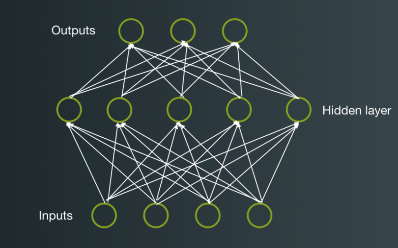
This gives rise to an infinity of possible network topologies:  How many intermediate (hidden) layers do you want?  How many nodes in each one?  There’s no need to apply the logistic function at each node; in principle, we can apply anything that our network framework can differentiate. So we could have a particular “activation function” for each layer or even for each node! Could we apply multiple activation functions?  Do we learn a weight for every single node in one layer to every single node in another, or do we skip some?

Add to this the usual parameters for gradient descent: Which algorithm to use?  How about the learning rate? Are we going to dropout training to avoid overfitting?  And let’s not even get into the usual parameters common to all ML algorithms, like how to handle missing data or objective weights. Whew!

Extra Credit

What we’ve described above is the vanilla feed-forward neural network that the literature has known for quite a while, and we can see that they’re pretty parameter heavy. To add a bit more to the pile, we’ve added support for a couple of fairly recent advances in the deep learning world (some of the “minor advances” mentioned by Russel) that I’d like to mention briefly.

Batch Normalization

During the training of deep neural networks, the activations of internal layers of the network can change wildly throughout the course of training. Often, this means that the gradients computed for training can behave poorly so one must be very careful to select a sufficiently low learning rate to mitigate this behavior.

Batch normalization fixes this by normalizing the inputs to each layer for each training batch of instances, assuring that the inputs are always mean-centered and unit-variance, which implies well-behaved gradients when training. The downside is that you must now know both mean and variance for each layer at prediction time so you can standardize the inputs as you did during training. This extra bookkeeping tends to slow down the descent algorithm’s per-iteration speed a bit, though it sometimes leads to faster and more robust convergence, so the trade-off can be worthwhile for certain network structures.

Learn Residuals

Residual networks are networks with “skip” connections built in. That is, every second or third layer, the input to each node is the usual output from the previous layer, plus the raw, unweighted output from two layers back.

The theory behind this idea is that this allows information present in the early layers to bubble up through the later layers of the network without being subjected to a possible loss of that information via reweighting on subsequent layers. Thus, the later layers are encouraged to learn a function representing the residual values that will allow for good prediction when used on top of the values from the earlier layers. Because the early layers contain significant information, the weights for these residual layers can often be driven down to zero, which is typically “easier” to do in a gradient descent context than to drive them towards some particular non-zero optimum.

Tree Embedding

When this option is selected, we learn a series of decision trees, random forest-style, against the objective before learning (with appropriate use of holdout sets, of course). We then use the predictions of the trees as generated “input features” for the network. Because these features tend to have a monotonic relationship with the class probabilities, this can make gradient descent reach a good solution more quickly, especially in domains where there are many non-linear relationships between inputs and outputs.

If you want, this is a rudimentary form of stacked generalization embedded in the tree learning algorithm.

Pay No Attention To The Man Behind The Curtain

So it seems we’ve set ourselves an impossible task here. We have all of these parameters. How on earth are we going to find a good network in the middle of this haystack?

Here’s where things get BigML easy:  the answer is that we’re going to do our best to find ones that work well on the dataset we’re given. We’ll do this in two ways:  via metalearning and via hyper-parameter search.

Metalearning

Metalearning is another idea that is nearly as old as Machine Learning itself.  In its most basic form, the idea is that we learn a bunch of classifiers on a bunch of different datasets and measure their performance. Then, we apply Machine Learning to get a model that predicts the best classifier for a given dataset. Simple, right?

In our application, this means we’re going to learn networks of every sort of topology parameterized in every sort of way. What do I mean by “every sort”?  Well, we’ve got over 50 datasets so we did five replications of 10-fold cross-validation on each one. For each fold, we learned 128 random networks, then we measured the relative performance of each network on each fold.  How many networks is that?  Here, allow me to do the maths:

50 * 5 * 10 * 128 = 320,000.

“Are you saying you trained 320,000 neural networks”  No, no, no, of course not!  Some of the datasets were prohibitively large so we only learned a paltry total of 296,748 networks.  This is what we do for fun here, people!

When we model the relative quality of the network given the parameters (which of course do use BigML), we learn a lot of interesting little bits about how the parameters of neural networks relate to one another and the data on which they’re being trained.

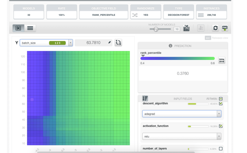
You’ll get better results using the “adadelta” decent algorithm, for example, with high learning rates, as you can see by the green areas of the figure below, indicating parts of the parameter space that specify networks, which perform better on a relative basis.

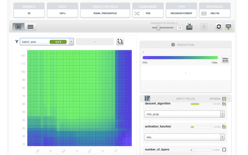
But if you’re using “rms_prop”, you’ll want to use learning rates that are several orders of magnitude lower.

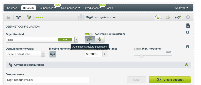
Thankfully, you don’t have to remember all of this.  The wisdom is in the model, and we can use this model to make intelligent suggestions about which network topology and parameters you should use, which is exactly what we do with the “Automatic Structure Suggestion” button.

But, of course, the suggested structure and parameters represent only a guess at the optimal choices, albeit an educated one.  What if we’re wrong?  What if there’s another network structure out there that performs well on your data, if you could only find it.  Well, we’ll have to go looking for it, won’t we?

Network Search

Our strategy here again comes in many pieces.  The first is Bayesian hyperparameter optimization.  I won’t go into it too much here because this part of the architecture isn’t too much more than a server-side implementation of SMACdown, which I’ve described previously. This technique essentially allows a clever search through the space of possible models by using the results of previously learned networks to guide the search. The cleverness here lies in using the results of the previously trained networks to select the best next one to evaluate. Beyond SMAC, we’ve done some experiments with regret-based acquisition functions, but the flavor of the algorithm is the same.

We’ve also more heavily parallelized the algorithm, so the backend actually keeps a queue of networks to try, reordering that queue periodically as its model of network performance is refined.

The final innovation here is using bits and pieces of the hyperband algorithm.  The insight of the algorithm is that a lot of savings in computation time can be gained by simply stopping training on networks that, even if their fit is still improving, have little hope of reaching near-optimal performance in reasonable time. Our implementation differs significantly in the details (in our interface, for example, you provide us with a budget of search time that we always respect), but does stop training early for many underperforming networks, especially in the later stages of the search.

This is all available right next door to the structure suggestion button in the interface.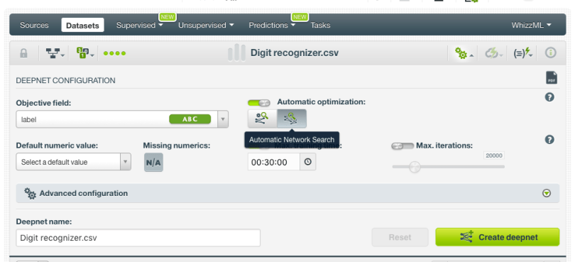Between metalearning and network search, we can make a good guess as to some reasonable network parameters for your data, and we can do a clever search for better ones if you’re willing to give us a bit more time.  It sounds good on paper, so let’s take it for a spin.

Benchmarking

So how did we do? Remember those 50+ datasets we used for metalearning?  We can use the same datasets to benchmark the performance of our network search against other algorithms (before you ask, no, we didn’t apply our metalearning model during this search as that would clearly be cheating). We again do 5 replications of 10-fold cross validation for each dataset and measure performance over 10 different metrics. As this was a hobby project I started before I came to BigML, you can see the result here.

You can see on the front page a bit of information about how the benchmark was conducted (scroll below the chart), and a comparison of 30+ different algorithms from various software packages. The thing that’s being measured here is “How close is the performance of this algorithm to the best algorithm for a given dataset and metric?”  You can quickly see that BigML Deepnets are the best thing or quite close more often than any other off-the-shelf algorithm we’ve tested.

The astute reader will certainly reply, “Well, yes, but you’ve done all manner of clever optimizations on top of the usual deep learning; you could apply such cleverness to any algorithm in the list (or a combination!) and maybe get better performance still!”

This is absolutely true.  I’m certainly not saying that BigML deep learning is the best Machine Learning algorithm there is; I don’t even know how you would prove something like that. But what these results do show is that if you’re going to just pull something off of the shelf and use it, with no parameter tuning and little or no coding, you could do a lot worse than to pull off BigML. Moreover, the results show that deep learning (BigML or otherwise; notice that multilayer perceptrons in scikit are just a few clicks down the list) isn’t just for vision and NLP problems, and it might be the right thing for your data too.

Another lesson here, editorially, is that benchmarking is a subtle thing, easily done wrong. If you go to the “generate abstract” page, you can auto-generate a true statement (based on these benchmarks) that “proves” that any algorithm in this list is “state-of-the-art”. Never trust a benchmark on a single dataset or a single metric! While any benchmark of ML algorithms is bound to be inadequate, we hope that this benchmark is sufficiently general to be useful.

Hopefully, all of this has convinced you to go off to see the Wizard and give BigML Deepnets a try. Don’t be the Cowardly Lion! You have nothing to lose except underperforming models…

Want to know more about Deepnets?

Please visit the dedicated release page for further learning. It includes a series of six blog posts about Deepnets, the BigML Dashboard and API documentation, the webinar slideshow as well as the full webinar recording.