The BigML Team has been working hard this summer to bring Deepnets to the platform, which will be available on October 5, 2017. As explained in our introductory post, Deepnets are an optimized implementation of the popular Deep Neural Networks, a supervised learning technique that can be used to solve classification and regression problems. Neural Networks became popular because they were able to address complex problems for a machine to solve like identifying objects in images.

The previous blog post presented a study case that showed how Deepnets can help you solve your real-world problems. In this post, we will take you through the five necessary steps to train a Deepnet that correctly identifies the digits using the BigML Dashboard. We will use a partial version of the well-known MNIST dataset (provided by Kaggle) for image recognition that contains 42,000 handwritten images of numbers from 0 to 9.

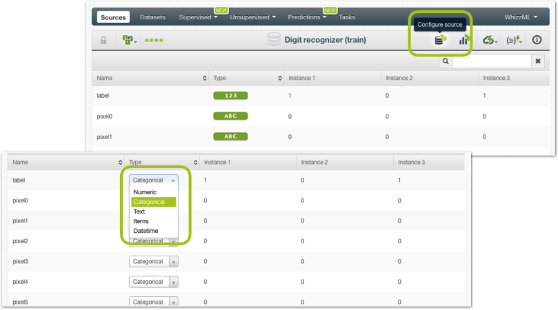
1. Upload your Data

As usual, you need to start by uploading your data to your BigML account. BigML offers several ways to do it, you can drag and drop a local file, connect BigML to your cloud repository (e.g., S3 buckets) or copy and paste a URL. This will create a source in BigML.

BigML automatically identifies the field types. In this case, our objective field (“label”) has been identified as numeric because it contains the digit values from 0 to 9. Since this is a classification problem (we want our Deepnet to predict the exact digit label for each image instead of a continuous numeric value), we need to configure the field type and select “Categorical” for our objective field.

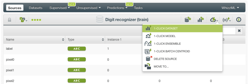
2. Create a Dataset

From your source view, use the 1-click dataset menu option to create a dataset, a structured version of your data ready to be used by a Machine Learning algorithm.

In the dataset view, you will be able to see a summary of your field values, some basic statistics, and the field histograms to analyze your data distributions. You can see that our dataset has a total of 42,000 instances and approximately 4,500 instances for each digit class in the objective field.

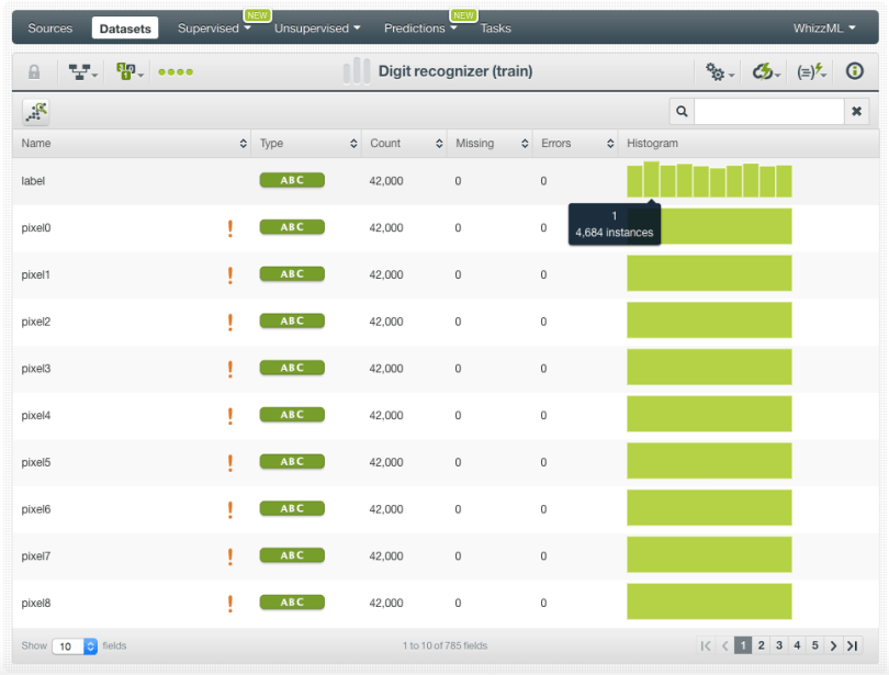
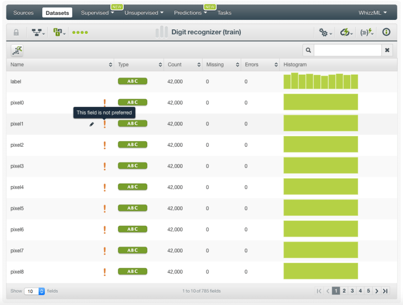
The dataset also includes a total of 784 fields containing the pixel information for each image. You can see that many fields are automatically marked as non-preferred in this dataset. This is because they contain the same value for all images so they are not good predictors for the model.

Since Deepnets are a supervised learning method, it is key to train and evaluate your model with different data to ensure it generalizes well against unseen data. You can easily split your dataset using the BigML 1-click action menu, which randomly sets aside 80% of the instances for training and 20% for testing.

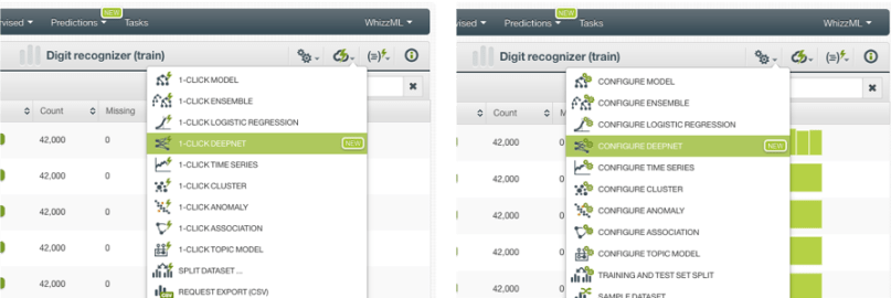
3. Create a Deepnet

In BigML you can use the 1-click Deepnet menu option, which will create the model using the default parameter values, or you can tune the parameters using the Configure Deepnet option.

BigML provides the following parameters to manually configure your Deepnet:

• Maximum training time and maximum iterations: you can set an upper bound to the Deepnet runtime by setting a maximum of time or a maximum number of iterations.
• Missing numerics and default numeric value: if your dataset contains missing values you can include them as valid values or replace them with the field mean, minimum, maximum or zero.
• Network architecture: you can define the number of hidden layers in your network, the activation function and the number of nodes for each of them. BigML also provides other three options related to how the layer connections are arranged such as residual learning, batch normalization and tree embedding (a tree-based representation of the data to input along with the raw features).
• Algorithm: you can select the gradient descent optimizer including Adam, Adagrad, Momentum, RMSProp, and FTRL. For each of these algorithms, you can tune the learning rate, the dropout rate and a set of specific parameters which explanation goes beyond the purpose of this post. To know more about the differences between algorithms you can read this article.
• Weights: if your dataset contains imbalanced classes for the objective field, you can automatically balance them with this option that uses the oversampling strategy for the minority class.

Neural Networks are known for being notoriously sensitive to the chosen architecture and the algorithm used to optimize the parameters thereof. Due to this sensitivity and the large number of different parameters, hand-tuning Deepnets can be difficult and time-consuming as the number of choices that lead to poor networks typically vastly outnumber the choices that lead to good results.

To combat this problem, BigML offers first-class support for automatic parameter optimization. In this case, we will use the automatic network search option. This option trains and evaluates over all possible network configurations, returning the best networks found for your problem. The final Deepnet will use the top networks found in this search to make predictions.

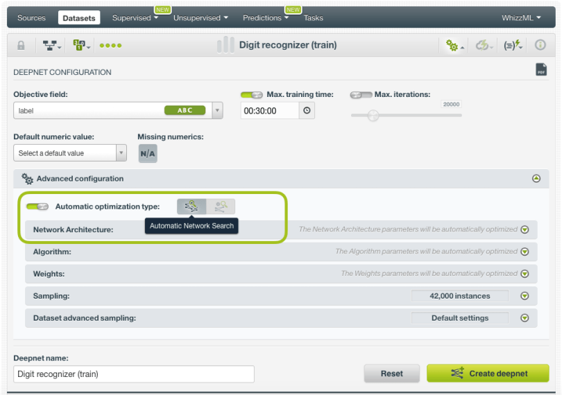
When the network search optimizer is enabled, the Deepnet creation may take some time to be created (so be patient!). By default, the maximum training time is set to 30 minutes, but you can configure it.

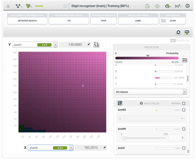
When your Deepnet is created you will be able to visualize the results in the Partial Dependence Plot. This unique view allows you to inspect the input fields’ impact on predictions. You can select two different fields for the axes and set the values for the rest of input fields to the right. You can see the predictions for each of the classes in different colors in the legend to the right by hovering the chart area. Each class color is shaded according to the class probability.

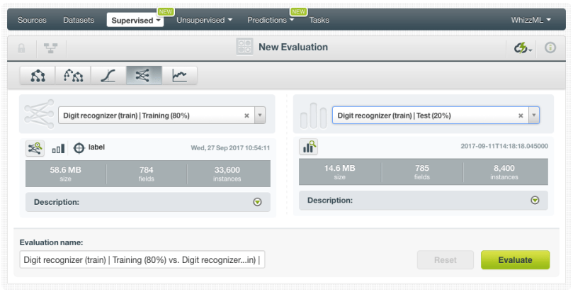
4. Evaluate your Deepnet

The Deepnet looks good, but we can’t know anything about the performance until we evaluate it. From your Deepnet view, click on the evaluate option in the 1-click action menu and BigML will automatically select the remaining 20% of the dataset that you set aside for testing.

You can see in the image below that this model has an overall accuracy of 96.1%, however, a high accuracy may be hiding a bad performance for some of the classes.

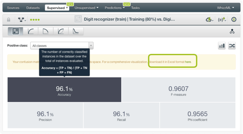
To look at the correct decisions as well as the mistakes made by the model per class we need to look at the confusion matrix, but we have too many different categories in the objective field and BigML cannot plot all them in the Dashboard, so we need to download the confusion matrix in Excel format.

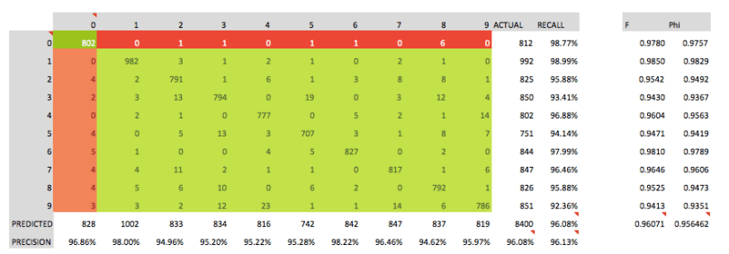
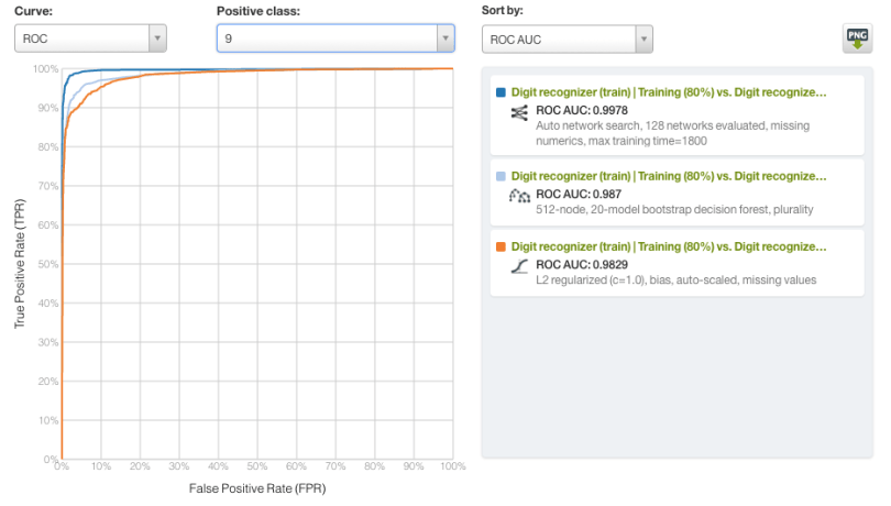
Ok, it seems we get very good results! In the diagonal of the table you can find the right decisions made by the model. Almost all categories have a precision and recall over 95%. Despite these great results, can they get better using other algorithms? We trained a Random Decision Forest (RDF) of 20 trees and a Logistic Regression to compare their performances with Deepnets. BigML offers a comparison tool to easily compare the results of different classifiers. We use the well-known ROC curve and the AUC as the comparison measure. We need to select a positive class, to make the comparison (in this case we selected the digit 9) and the ROC curves for each model are plotted in the chart. You can see in the image below how our Deepnet outperforms the other two models since its ROC AUC is higher.

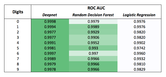
Although RDF also provides pretty good results, the ROC AUC for Deepnets is consistently better for all the digits from 0 to 9 as you can see in the first column in the table below.

5. Make Predictions using your Deepnet

Predictions work for Deepnets exactly the same as for any other supervised method in BigML. You can make predictions for a new single instance or multiple instances in batch.

Single predictions

Click on the Predict option from your Deepnet view. A form containing all your input fields will be displayed and you will be able to set the values for a new instance. At the top of the view, you will get all the objective class probabilities for each prediction.

Since this dataset contains more than 100 fields, we cannot perform single predictions from the BigML Dashboard, but we can use the BigML API for that.

Batch predictions

If you want to make predictions for multiple instances at the same time, click on the Batch Prediction option and select the dataset containing the instances for which you want to know the objective field value.

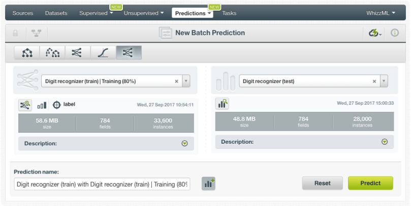
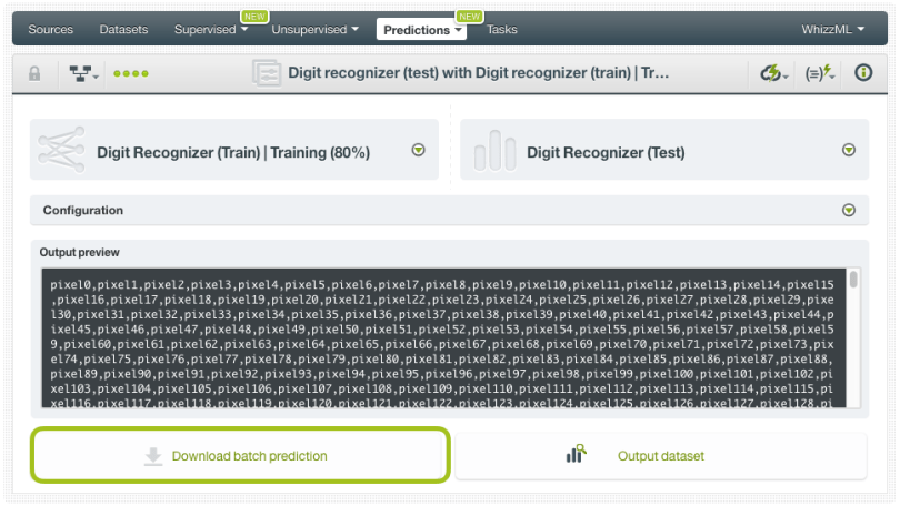
You can configure several parameters of your batch prediction like the possibility to include all class probabilities in the output dataset and file. When your batch prediction finishes, you will be able to download the CSV file and see the output dataset.

Want to know more about Deepnets?

Stay tuned for the next blog post, where you will learn how to program Deepnets via the BigML API. If you have any questions or you’d like to learn more about how Deepnets work, please visit the dedicated release page. It includes a series of six blog posts about Deepnets, the BigML Dashboard and API documentation, the webinar slideshow as well as the full webinar recording.