Even Easier Machine Learning for Every Day Tasks

Recently, the “Machine Learning for Everyday Tasks” post suddenly rising to the top of Hacker News drew our attention. In that post, Sergey Obukhov, software developer at San Francisco-based startup Mailgun, tries to debunk the myth that Machine Learning is a hard task:

I have always felt like we can benefit from using machine learning for simple tasks that we do regularly.

This certainly rings true to our ears at BigML, since we aim to democratize Machine Learning by providing developers, scientists, and business users powerful higher-level tools that package the most effective algorithms that Machine Learning has produced in the last two decades.

In this post, we are going to show how much easier it is to solve the same problem tackled in the Hacker News post by using BigML. To this end, we have created a test dataset with similar properties to the one used in the original post so that we can replicate the same steps with analogous results.

Predicting processing time

The objective of this analysis is predicting how long it will take to parse HTML quotations embedded within e-mail conversations. Most messages are processed in a very short time, while some of them take much longer. Identifying those lengthier messages in advance is useful for several purposes, including load-balancing and giving more precise feedback to users.

Our analysis is based on a CSV file containing a number of fictitious track records of our system performance when handling email messages:

HTML length, Tag count, Processing Time

We would like to classify a given incoming message as either slow or fast given its length and tag count based on previously collected data.

Finding a definition for slow and fast through clustering

The first step in our analysis is defining what slow and fast actually mean. The approach in the original post is clustering, which identifies groups of relatively homogeneous data points. Ideally, we would hope that this algorithm is able to collect all slow executions in one cluster and all fast executions in another.

In the original post, the author has written a small program to calculate the optimal number of clusters. Then he uses that number as a parameter to actually build the clusters.

The task of estimating the number of clusters to look for is so common that BigML provides a ready-made WhizzML script that does exactly that: Compute best K-means Clustering. Alternatively, BigML also provides the G-means algorithm for clustering, which is able to automatically identify the optimal number of clusters. For our analysis, we will use the Compute best K-means Clustering script, following these steps:

1. Create a dataset in BigML from your CSV file
2. Execute the Compute best K-means clustering script using that dataset.

We can carry out those steps in a variety of ways, including:

• Using BigML Dashboard, which makes it really easy to investigate a problem and build a machine learning solution for it in a pointing and click manner.
• Writing a program that uses BigML REST API and the proper bindings that BigML provides for a number of popular languages, such as Python, Node.js, C#, Java, etc.
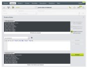
• Using bigmler, a command-line tool, which makes it easier to automate ML tasks.
• Using WhizzML, a server-side DSL (Domain Specific Language) that makes it possible to extend the BigML platform with your custom ML workflows.

We are going to use the BigML bindings for Python as follows:

import webbrowser
from bigml.api import BigML

api = BigML()

source = api.create_source('./post-data.csv')
dataset = api.create_dataset(source)
api.ok(dataset)
print "dataset" + dataset['resource']
execution = api.create_execution('script/57f50fb57e0a8d5dd200729f',
                                 {"inputs": [
                                     ["dataset", dataset['resource']],
                                     ["k-min", 2],
                                     ["k-max", 10],
                                     ["logf", True],
                                     ["clean", True]
                                 ]})
api.ok(execution)
best_cluster = execution['object']['execution']['result']
webbrowser.open("https://bigml.com/dashboard/" + best_cluster)

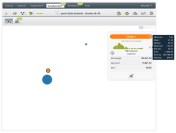
The result tells us that we have:

• Two clusters (green and orange) that contain definitely slow instances.

• The blue cluster includes the majority of instances, both fast and not-so-fast, as its statistical distribution in the cluster detail panel indicates:

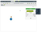
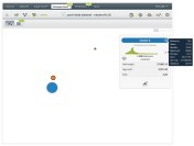
Seemingly, our threshold to distinguish fast tasks from slow tasks points to the green cluster.

At this point, the original post gives up on using clustering as a means to determine a sensible threshold, and reverts to plotting time percentiles against tag count. Luckily for them, the percentile distribution shows a nice bubbling up at the 78th percentile, but in general this kind of analysis may not always yield such obvious distributions. As a matter of fact, detecting such an abnormalities can be even harder with multidimensional data.

BigML makes it very simple to further investigate the properties of the above green cluster. We can simply create a dataset including only the data instances belonging to that cluster and then build a simple model to better understand its characteristics:

centroid_dataset = api.create_dataset(best_cluster, { 'centroid' : '000000' })
api.ok(centroid_dataset)

centroid_model = api.create_model(centroid_dataset)
api.ok(centroid_model)

webbrowser.open("https://bigml.com/dashboard/" + centroid_model['resource'])

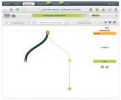
This, in turn, produces the following model:

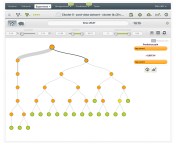
If you inspect the properties of the tree nodes, you can see that the tree is clearly quickly split into two subtrees with all nodes on the left-hand subtree having processing times lower than 14.88 sec, and all nodes belonging to the subtree on the right with processing times greater than 16.13.

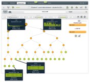
This suggests that a good choice for the threshold between fast and slow can be approximately 15.5 sec.

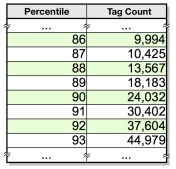
If we follow along the same steps as in the original post and apply the percentile analysis to our data instances here, we arrive at the following distribution:

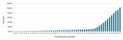
This distribution clearly starts growing faster between the 88th to the 89th percentile, confirming our choice of threshold:

To summarize, we have found a comparable result by applying a much more generalizable analysis approach.

Feature engineering

With the proper threshold identified, we can mark all data instances with running times lower than 15.5 as fast and the rest as slow. This is another task that BigML can tackle easily via its built-in feature engineering capabilities on BigML Dashboard:

Alternatively, we do the same in Python:

extended_dataset = api.create_dataset(dataset, {
    "new_fields" : [
        { "field" : '(if (< (f "time") 15.5) "fast" "slow")',
          "name" : "processing_speed" }]})

webbrowser.open("https://bigml.com/dashboard/" + extended_dataset['resource'])

Which produces the following dataset:

Predicting slow and fast instances

Once we have all our instances labeled a fast and slow, we can finally build a model to predict whether an unseen instance will be fast and slow to process. The following code creates the model from our extended_dataset:

extended_dataset = api.create_dataset(dataset, {
   "excluded_fields" : ["000002"],
    "new_fields" : [
        { "field" : '(if (< (f "time") 15.5) "fast" "slow")',
          "name" : "processing_speed" }]})
api.ok(extended_dataset)
webbrowser.open("https://bigml.com/dashboard/" + extended_dataset['resource'])

Notice that we excluded the original time field from our model, since we are now relying on our new feature that tells apart the fast instances from slow ones. This step yields the following result that shows a nice split between fast and slow instances at around 9,589 tags (let’s call this _MAX_TAGS_COUNT):

Admittedly, our example here is pretty trivial. As was the case in the original post, our prediction boils down to this conditional:

def html_too_big(s):
    return s.count(' _MAX_TAGS_COUNT

But, what if our dataset were more complex and/or the prediction involved more intricate calculations? This is another situation, where using a Machine Learning platform such as BigML provides an advantage over an ad-hoc solution. With BigML, predicting is just a matter of calling another function provided by our bindings:

from bigml.model import Model

final_model = "model/583dd8897fa04223dc000a0c"
prediction_model = Model(final_model)
prediction1 = prediction_model.predict({
    "html length": 3000,
        "tag count": 1000 })
prediction2 = prediction_model.predict({
    "html length": 30000,
        "tag count": 500 })

What’s more, predictions are fully local, which means no access to BigML servers is required!

Conclusion

Machine Learning can be used to solve everyday programming tasks. There are certainly different ways to do that, including tools like R and various Python libraries. However, those options have a steeper learning curve to master the details of the algorithms inside as well as the glue code to make them work together. One must also take into account the need to maintain and keep alive such glue code that can result in considerable technical debt.

BigML, on the other hand, provides practitioners all the tools of the trade in one place in a tightly integrated fashion. BigML covers a wide range of analytics scenarios including initial data exploration, fully automated custom Machine Learning workflows, and production deployment of those solutions on large-scale datasets. A BigML workflow that solves a predictive problem can be easily embedded into a data pipeline, which unlike R or Python libraries does not require any desktop computational resources and can be reproduced on demand.