The Neural Information Processing Systems (NIPS) conference is one of the most important events in Machine Learning. It receives hundreds of papers from researchers all over the world each year. On the occasion of the NIPS conference held in Barcelona last week, Kaggle published a dataset containing all NIPS papers between 1987 and 2016.
We found it an excellent opportunity to put BigML’s latest addition in practice: Topic Models.
Assuming that paper topics evolve gradually over the years, our main goal in this post will be to predict the decade in which the papers were published by using their topics as inputs. Then, by examining the resulting model, we can get a rough idea of which research topics are popular now, but not in the past, and vice-versa.
We will accomplish this in four steps: first, we will transform the data into a Machine Learning-ready format; second, we will create a Topic Model and inspect the results; then, we will add the resulting topics as input fields; finally, we will build the predictive model using the decade as the objective field.
1. The Data
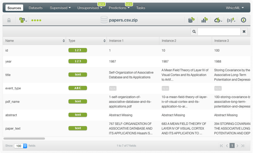
We start by uploading the CSV file “papers” to BigML. BigML creates a source while automatically recognizing the field types and showing a sample of the instances so we can check that the data has been processed correctly. As you can see below, the source contains the title, the authors, the year, the abstracts and the full text for each paper.
Notice that BigML supports compressed files such as .zip files so we don’t need to decompress the source file first. Moreover, BigML automatically performs some text analysis that also aids Topic Models (e.g., tokenization, stemming, stop words and case sensitivity cleaning) so you don’t need to worry about any text pre-processing. You can read more about the text options for Topic Models here.
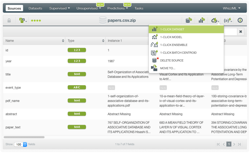
When the source is ready, we can create a dataset, which is a structured version of your data interpretable by a Machine Learning model. We do this by using the 1-click option shown below.
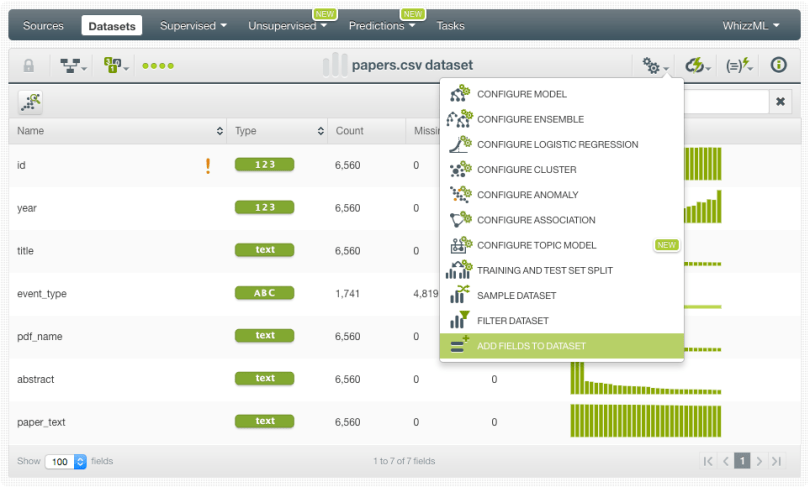
Since we want to predict the publication decade of the NIPS papers, we need to transform the “year” into a categorical field. This field will include four different categories: 80s, 90s, 2000s and 2010s. We can easily do so by clicking the option “Add fields to dataset”.
Then we need to select “Lisp s-expression” and use the Flatline editor to calculate the decade using the “year” field. We will not cover all the steps to create a field using the Flatline editor, but you can find a detailed explanation in Section 9.1.7 of the datasets document.

The formula we need to insert contains several “If…” statements to group years into decades:
(if (< (f "year") 1990) "80s" (if (< (f "year") 2000) "90s" (if (< (f "year") 2010) "2000s" "2010s")))
When the new field is created, we can find as the last field in the dataset. By mousing over the histogram we can see the different decades:

2. Discovering the Topics Underlying the NIPS Papers
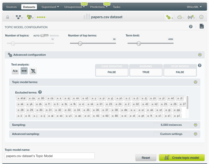
Creating a Topic Model in BigML is very easy. You can either use the 1-click option or you can configure the parameters. To discover the topics for the NIPS papers, we are going to configure the following parameters:
- Number of top terms: by default, BigML shows top 10 terms per topic. We prefer set a higher limit this time, up to 30 terms, so we can have more terms glean the topic themes from.
- Bigrams: we include bigrams in the Topic Model vocabulary since we expect the NIPS reports to show a high number of them, e.g., neural networks, reinforcement learning or computer vision.
- Excluded terms: we exclude terms such as numbers and variables since they are not significant in delimiting the papers’ thematic boundaries over time and can generate some noise.
When the Topic Model is created, you can inspect the topic terms using two different visualizations: the topic map and the term chart. See both in the images below.
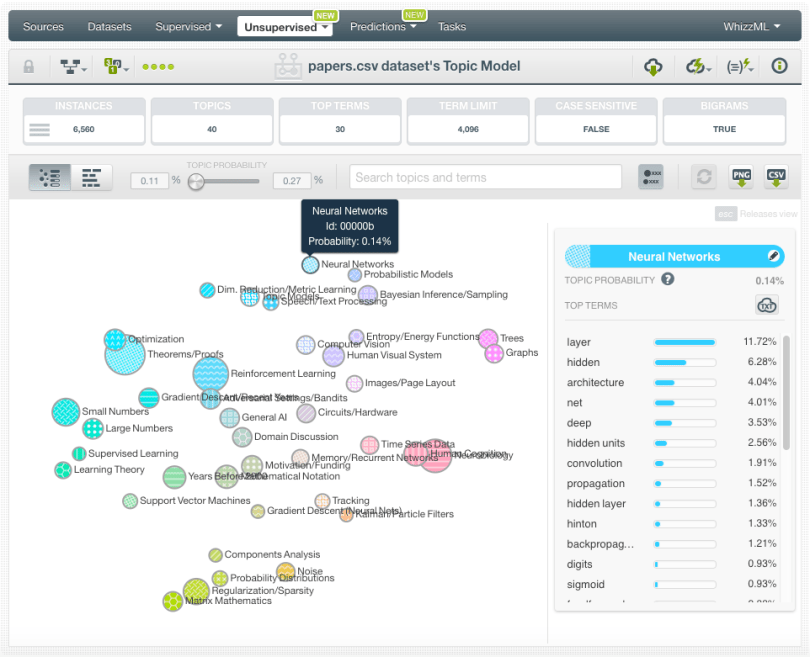
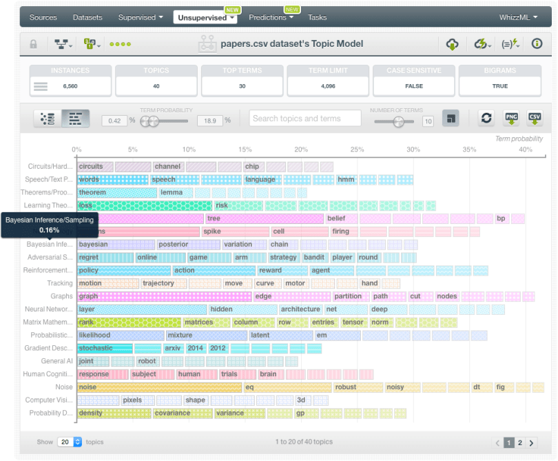
You can see the resulting Topic Model and play with the associated BigML interactive visualizations here!
The discovered topics provide a nice overview of most of the major subtopics in Machine Learning research, and we’ve renamed them to make them readable at a glance. In the “north” of the topic model map, we have topics related to Bayesian and Probabilistic modeling, along with Text/Speech processing and computer vision, which represent domains where those techniques are popular. In the “south”, we get the topics that are heavily tilted towards matrix mathematics, including PCA and the specification of multivariate Gaussian probabilities. In the “west” we have supervised learning and optimization, with topics containing theorem proving along with various occurrences of numbers in this quadrant. In the “east” we have two rather isolated topics corresponding to data structures, specifically trees and graphs. Finally, in the center of the map, we have topics that occur across every discipline: General AI terms (like “robot”), people talking about the real-world domain that they’re working in, and acknowledgements for collaborators and funding.
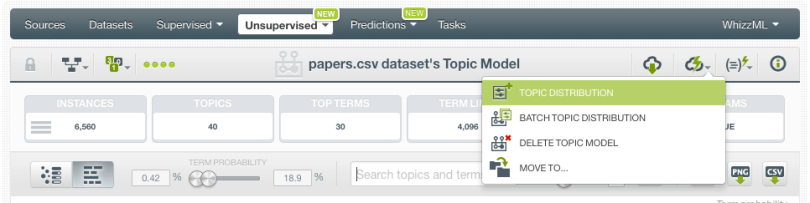
With the topics discovered, let’s try to predict the topic distribution for a new document. A good way to visually analyze the Topic Model predictions is to use BigML Topic Distributions. You can use the corresponding option within the 1-click menu:
A form containing the fields used to create the Topic Model will be displayed so you can insert any text and get the topic distributions.
We input the following data for our first Topic Distribution:
- Title: “Deep Learning Models of the Retinal Response to Natural Scenes”
- Abstract: “A central challenge in sensory neuroscience is to understand neural computations and circuit mechanisms that underlie the encoding of ethologically relevant, natural stimuli. (..) Here we demonstrate that deep convolutional neural networks (CNNs) capture retinal responses to natural scenes nearly to within the variability of a cell’s response, and are markedly more accurate than linear-nonlinear (LN) models and Generalized Linear Models (GLMs). (…) the injection of latent noise sources in intermediate layers enables our model to capture the sub-Poisson spiking variability observed in retinal ganglion cells. (..) Overall, this work demonstrates that CNNs not only accurately capture sensory circuit responses to natural scenes, but also can yield information about the circuit’s internal structure and function.”
The resulting topics, in the order of importance, include: Human Visual System (22.15%), Neurobiology (19.89%), Neural Networks (10.77%), Human Cognition (8.72%), Computer Vision (6.96%), Noise (5.17%) among others with lower probabilities. You can see the resulting probabilities histogram in the image below:

After making several predictions for different papers, we’re pretty confident that the predictions map fairly well with the judgements a human expert might make. Give it a try for yourself with this Topic Model link!
3. Including Topics as Input Fields
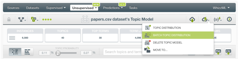
At this point, we know that the resulting topics are consistent and the model satisfactorily calculates the different Topic Distributions for the papers. Now, we can try using the topic distribution to predict when the paper was written.
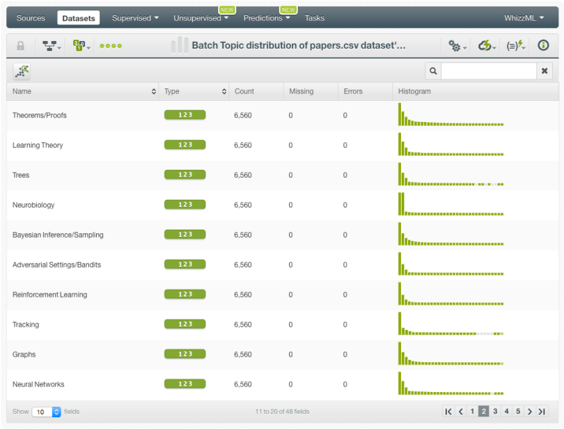
In order to incorporate the different Topic Distributions for all the papers in the dataset, we need to click in the “Batch Topic Distribution” option and select the dataset that contains the field “decade”(the field we created in the first step above).
When the Batch Topic Distribution is created, we can find the resulting dataset containing all the topic distributions as fields.
4. Predicting a Paper’s Decade
Finally, we are ready to build a model to predict any paper’s decade using the topics as inputs.
We first need to split the dataset into training and testing subsets randomly. In this case, we are going to use 80% of the dataset to build a Logistic Regression. For this, we remove all fields except the topics and the paper abstract and select the decade as the objective field.
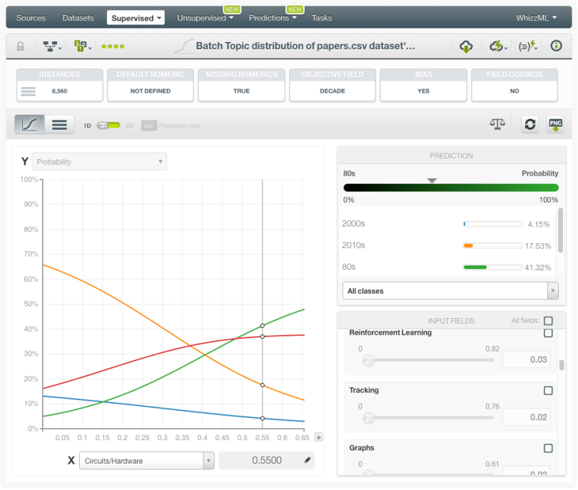
BigML visualizations for Logistic Regression allow us to interpret the most influencing topics to predict the decade. By selecting a topic for the x-axis of the Logistic Regression chart, we can see the most sensitive topics that evolve over time vs. the most stable topics. The fluctuating topics will be better predictors of the decades than the more steady topics, which will be mostly irrelevant for our supervised model.
For example, we can see in the image below that as the probability for the topic “Circuits/Hardware” increases, it is more likely to appear in the papers from the 80’s and 90’s than in the papers from the 21st century. Therefore, it can be an important topic in determining which decade a paper was written.
The topic “Support Vector Machines” for example, tend to be very frequent in papers from the 2000’s while it is less probable in other decades.
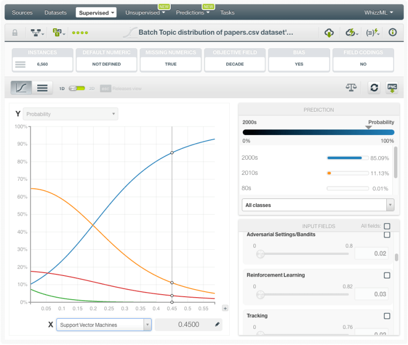
Other topics like “Small numbers” (which includes all the numbers found in the papers) or “Probabilistic Distributions” tend to have a stable probability throughout all the decades. You can observe this in the image below, where the graph lines are pretty flat, i.e., the predicted probabilities for the decades do not change per topic probabilities.


The results seem to fit nicely vs. our expectations, but to objectively measure the overall predictive power of this model, we need to evaluate it by using the remaining 20% of the data.
The Logistic Regression evaluation shows around 80% accuracy, which is not bad. However, after trying other classification models, we find out that the best performing model is a Bagging ensemble of 300 trees, which achieves an accuracy of 84%. You can see its confusion matrix below.
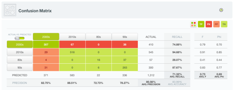
In here, we see the most difficult decade to predict for is the 80’s, very likely due to a smaller number of papers (57 in total) in the sample as compared to the other decades.
To improve the model performance further, we can try some more Feature Engineering such as the length of the text, the authors, the number of papers from the authors, various extracted entities like the university/country published in.
We encourage you to delve in to this fun dataset, and let us know of ways to improve it. If you haven’t got a BigML account yet, it’s high time you get one today. Sign up now, it’s free!
