WhizzML Tutorial II: Covariate Shift

If this is your first time writing in the new WhizzML language, I suggest that you start here with a more simple tutorial. In this post, we are going to write a WhizzML script that automates the process of investigating Covariate Shift. To get a deeper understanding of what we’re trying to do, read the beginning of this article first.

We want a workflow that:

1. Given two datasets (one that represents the data used to train a predictive model, one that represents production data)
2. Returns an indication of whether the distribution of data is different between the two datasets

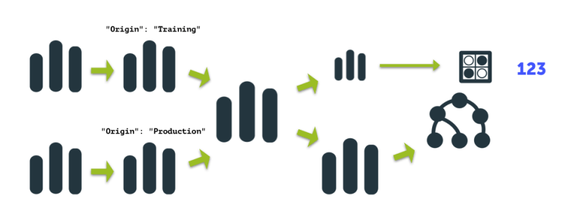
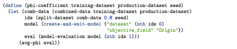
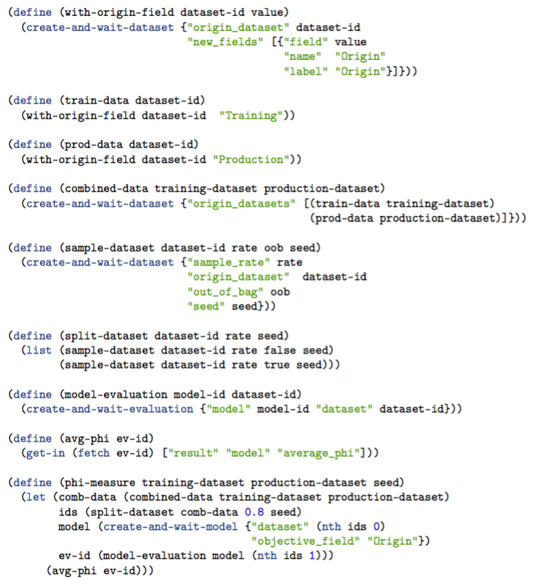
As we read in the article (or on Wikipedia), the indicator of change in our data distribution is called the phi coefficient. Our WhizzML script will return us this number, so let’s name our base function phi-coefficient.

phi-coefficient

What are we doing here?

To start, the function takes three arguments. The first two are ids for our training and production datasets, respectively. We call them training-dataset and production-dataset. The third argument, seed, is used to make our sampling deterministic. We’ll talk about this later.

There’s quite a bit going on in this function, but it’s all broken into manageable pieces. First, we use let to set local variables. These local variables are the result of a few different functions, which we will have to define. The local variables are comb-data, ids, model, and eval. After these are set, we can compute the phi coefficient with the function avg-phi. Let’s go over each of the local variables.

comb-data

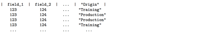
comb-data is the result of (combined-data training-dataset production-dataset). Here, we combine the two datasets into one big dataset. But before they are combined, we have to do a transformation on each dataset (add the “Origin” field). We’ll talk about that transformation when we define combined-data.

The dataset returned by our comb-data function looks something like this:

ids

Next, we have a variable called ids. This is a list of two dataset IDs – the result of:

Our split-dataset function takes the comb-data (one big dataset) and randomly splits it into two datasets. We split it so that we can train a predictive model with the larger portion of the split, and then evaluate its performance on the smaller part. The split-dataset function returns something like this:

["dataset/83bf92b0b38gbgb" "dataset/83hf93gf012bg84b20"]

model

model is a BigML predictive model resource. We are creating this model from the first element of our ids list: "dataset" (nth ids 0). The model is built to predict whether the value for the “Origin” field is “Training” or “Production”. Thus, the “objective_field” is “Origin”: "objective_field" "Origin".

eval

eval is a BigML evaluation resource. To create an evaluation, we need two arguments: a predictive model and a dataset we want to test the model against. Our model is stored in model and our dataset is the second element in the ids list, hence: (nth ids 1)

avg-phi

We’re done with the local variables, but what does the whole phi-coefficient function return – what’s our end product?

That line gives us the average phi score for the evaluation we just created. A bunch of information is stored inside the eval data object that will be retrieved from BigML. But of course we have to tell the function avg-phi how to get what we want! We’ll save that for later.

So we have built our base function (phi-coefficient)and understand its components. Now we have to go back and build the functions we haven’t defined yet, specifically comb-data, split-dataset, model-evaluation and avg-phi. We’ll start with comb-data.

comb-data

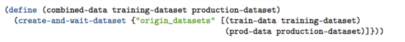
Again, this function combines two datasets. We tell BigML what datasets we want to combine using the “origin_datasets” parameter and passing it a list of dataset ids.

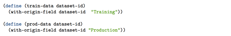
But what are train-data and prod-data?

Those are helper functions that add the “Origin” field we talked about.

• train-data adds the “Origin” field with the value “Training” in each row
• prod-data adds the “Origin” field with the value “Production” in each row

They are defined here:

Since we are doing pretty similar things in both functions, (adding an “Origin” field) we can separate that logic into its own function. Here it is:

with-origin-field

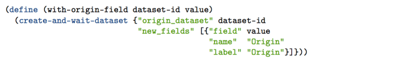
In that function we are…

1. Creating a new dataset from an existing one "origin_dataset" dataset-id
2. Adding a new field "new_fields" [...]
3. Giving the new field a column name and label "name" "Origin" "label" "Origin"
4. Setting the row’s value "field" value

The value will either be the string "Production" or "Training". This string is passed in as an argument where prod-data and train-data are defined.

Nice. Nows let’s go over split-dataset.

split-dataset

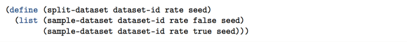
1. What are we splitting? dataset-id – the dataset we pass in.
2. How are we splitting it, 80%/20%? 90%/10%? We can do whatever we want. This is determined by rate.
3. How are we going to shuffle our data before we split it? The seed determines this.

As you can see, we are sampling the same dataset twice. One sample will be used to build a predictive model, the other will be used to evaluate the predictive model.

sample-dataset is another function. Here it is below:

sample-dataset

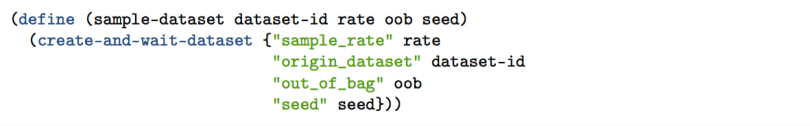
This function interacts with the BigML API. We create a new dataset, passing in the rate, the original dataset (dataset-id), whether it is out_of_bag or not (we’ll go over this) and the seed used to determine how the original dataset was shuffled.

Here’s a little diagram that will help explain how the seed and out_of_bag (oob) work.

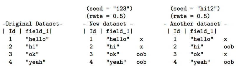
So if out_of_bag is set to true, we grab the rows labeled “oob”. Otherwise, we grab the ones marked “x”. The seed just changes which rows we label “oob” and “x”. The seed also enables this whole process be deterministic. So if you run the phi-coefficient function with the same seed (and the same datasets), you’ll get the same results!

Cool. That wraps up our split-dataset function. Next up, model-evaluation.

model-evaluation

I apologize if you were hoping for something more exciting. This function is just a wrapper for the method included with WhizzML, create-and-wait-evaluation. As you can see, we are simply creating an evaluation with a model and a dataset. Our last function is…

avg-phi

Pretty simple too!

We take the evaluation ev-id and fetch its data from BigML (fetch ev-id). Then we access the “average_phi” attribute nested under “model” and “result”. The data object looks like this:

And there we have it. A WhizzML script that helps predict Covariate shift.

All together:

We can run our function like this:

But…

As we read in the previous post, it is best to do this process several times and look at the average of the results. How could we add some more code to to do this programmatically? Here’s one implementation.

multi-phis

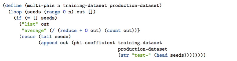
Again, we are giving this function our training-dataset and production-dataset. But we are also passing in n, which is the number of phi-coefficients we want to calculate. As you can see, we are defining a loop.

Within this loop, we set some variables.

seeds, we give the default (starting) value of (range 0 n). If we pass in 4 for the value of n then the initial value of seeds = [0 1 2 3]

out is our output. We will add the result of a phi-coefficient run each time through the loop. Initially, out = []

We also define the end-scenario.

seeds = (tail seeds). This grabs everything but the first element of seeds. So the first time through, it might be [0 1 2 3], then it will be [1 2 3], then [2 3]…

If seeds is not empty, we go back to the loop, but define values for seeds and out.

If seeds is empty, then we return a map with the values list and average (we’ll explain these in a bit).

out = (append out (phi-coefficient ...)) We take the result of our phi-coefficient function and add it to the out list. The first time through, it’s [], then [-0.0838], then [-0.0838, 0.1240] etc.

The seed we will use for each of these phi-coefficient runs will be "test-0", "test-1", "test-2" etc.  Thats what (str "test-" (head seeds)) is doing – joining the string "test-" with the first element of the seeds list.

The last thing we should discuss is the end-case return value:

The value of “list” (out) is just the list of phi-coefficient values from each run. The “average” is… Yep. The average of all the runs.reduce adds up the elements. count counts the number of elements. / divides the first argument by the second. That’s it!*

Example run:

We have now automated the process to investigate whether our distribution of data has changed. Great! You might want to create a scheduled job to check your production data against the data you used to create a predictive model. When the covariate shift exceeds a threshold, retrain the model!

Why WhizzML?

Wait… couldn’t we already do this with the API bindings? What’s special about WhizzML?

Yes, we could use the API bindings. However, there are two significant advantages to WhizzML. First, what if we write this workflow in Python and later decide we want to do the same thing workflow in NodeJS app? We would have to rewrite it the whole workflow!  WhizzML lets us codify our workflow once and use it from any language. Second, WhizzML removes the complexity and brittleness of needing to send multiple HTTP requests to the BigML server (for creating intermediate resources, fetching data, etc.). One HTTP request is all you need  to execute a workflow with WhizzML.

Stay tuned for more blog posts like this that will help you get started automating your own Machine Learning workflows and algorithms.

---

*There is actually one more thing we can do: a performance enhancement. In each phi-measure run, we recreate the train-data , prod-data and comb-data datasets. This is unnecessary – we can reuse the comb-data dataset and just sample it differently for each run! You can check out the code that includes this improvement here. Note that the comb-data logic from the phi-coefficient function is moved into the loop of multi-phis , and thus the phi-coefficient function is renamed to sample-and-score.