Looking for Connections in Your Data – Correlation Coefficients

This is part of an ongoing statistics-related blog post series in anticipation of BigML’s upcoming statistical tests resource. The previous post was about fraud detection with Benford’s Law. In this post, we will explore the topic of correlation, and how it can help you in designing and applying machine learning models.

Consider the following…

Put in plain terms, correlation is a measure of how strongly one variable depends on another. Consider a hypothetical dataset containing information about professionals in the software industry. We might expect a strong relationship between age and salary, since senior project managers will tend to be paid better than young pup engineers. On the other hand, there is probably a very weak, if any, relationship between shoe size and salary. Correlations can be positive or negative. Our age and salary example is a case of positive correlation. Individuals with a higher age would also tend to have a higher salary. An example of negative correlation might be age compared to outstanding student loan debt: typically older people will have more of their student loans paid off.

Correlation can be an important tool for feature engineering in building machine learning models. Predictors which are uncorrelated with the objective variable are probably good candidates to trim from the model (shoe size is not a useful predictor for salary). In addition, if two predictors are strongly correlated to each other, then we only need to use one of them (in predicting salary, there is no need to use both age in years, and age in months). Taking these steps means that the resulting model will be simpler, and simpler models are easier to interpret.

There are many measures for correlation, but by far the most widely used one is Pearson’s Product-Moment coefficient, or Pearson’s r. Given a collection of paired (x,y) values, Pearson’s coefficient produces a value between -1 and +1 to quantify the strength of dependence between the variables x and y. A value of +1 means that all the (x,y) points lie exactly on a line with positive slope, and inversely, a value of -1 means that all of the points lie exactly on a line with negative slope. A Pearson’s coefficient of 0 means that there is no relationship between the two variables. To see this visually, we can look at plots of our hypothetical data, and the Pearson’s coefficient computed from them.

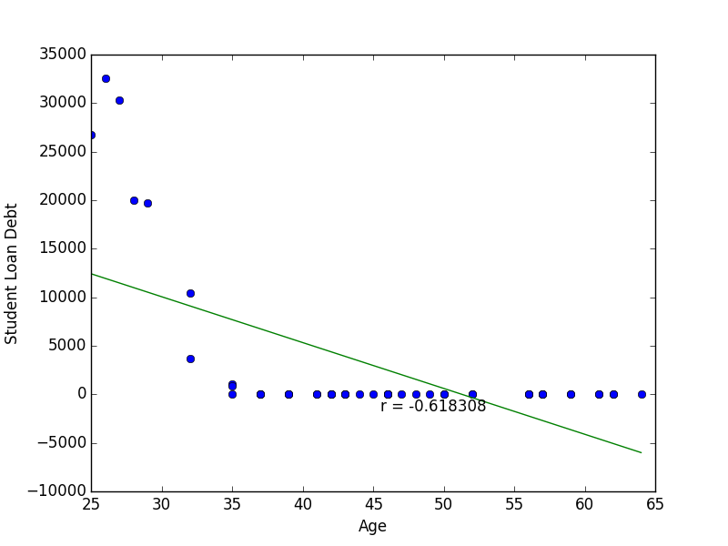
We observe that the sign of the correlation coefficient matches the slope of the line of best fit. Note, however that the magnitude of the coefficient is not related to the slope of the line, but only on how well the points fit the line. Also notice from our Age vs. Debt plot that the relationship between the two variables is more exponential rather than linear. Despite seeing a clear relationship between the two variables, a good straight line fit can not be made and so the resulting correlation coefficient is smaller than one might expect. To elaborate on how non-linear data can confound Pearson’s r, we turn our attention to Anscombe’s Quartet. This is a set of four cleverly constructed datasets which have the same Pearson’s correlation coefficient, as well as other summary statistics, yet are significantly dissimilar when seen on a graph.

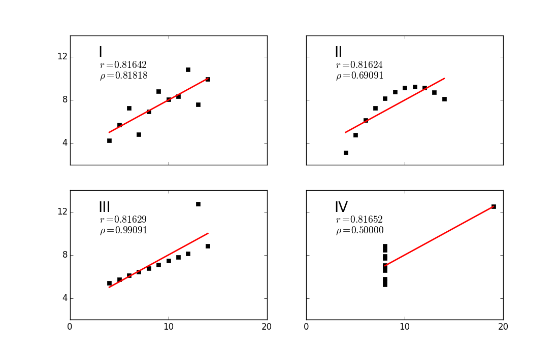
In cases such as this, Spearman’s rank-correlation coefficient, or Spearman’s rho, may be a good alternative measure. Spearman’s rho quantifies how monotonic the relationship between the two variables is, i.e. “Does an increase in x usually result in an increase in y?” (technically it is equivalent to computing Pearson’s r for a rank-transformed version of the data). We can see that while the four Anscombe datasets have equivalent Pearson’s r, Spearman’s rho does a good job discriminating them.

Correlation coefficients are a useful tool for exploring relationships within your data. Having been introduced to the topic of correlations, we invite you explore it further with BigML’s new correlations resource, and start exploring your data!