Predicting with My Model: Is It Safe?

“Remember that all models are wrong; the practical question is how wrong do they have to be to not be useful.” (George E.P. Box) If you – like me – have no modeling and machine learning background, it is a bit of a paradigm shift to appreciate that all models are wrong. Why on earth create a model if you know a priori it is wrong? Well, as my co-author for this post Charlie Parker taught me, because they still can be useful and improve your performance! As long as you take into account that predictions are not a future truth but rather represent the likelihood of something happening.

So how wrong is your model?  Or better yet, how right is it?  There’s no need to subject your model to dentistry-based coersion to find out if it’s safe to make predictions from it; you can now easily evaluate your model within BigML on any data you have.  In its simplest form, this is a three-click process:

1. Click the ‘Evaluate’ action for a Model
2. Select the Dataset you want to use to evaluate your Model
3. Click ‘Evaluate’.

Let’s look into that a bit closer.

You have just created a Model with a great Dataset. The official term is that you have ‘trained a Model’ and the data you used is called your training data. To evaluate how good this Model predicts, you need a similar, second set of data. Just like your training data, this set includes the value of the objective feature. This is called your test data. As with any data, you have uploaded your test data and created a BigML Dataset. It is this test data Dataset that you enter in the searchbox to select for your evaluation. BigML can now make predictions for every instance in the test data and compare the predicted outcome to the actual value in your test data. This forms your evaluation.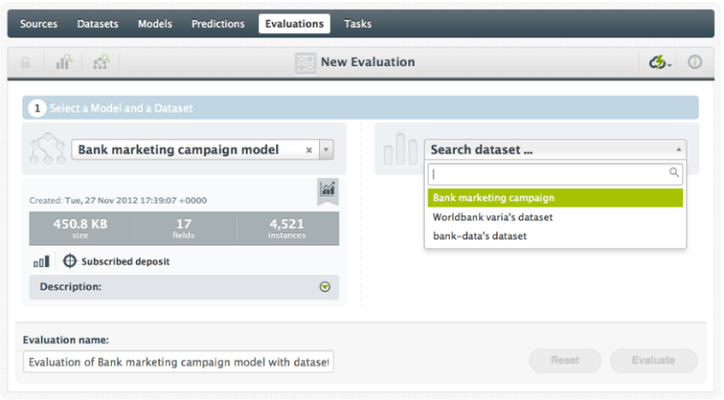

Can you use your training data as test data? Technically you can, but that’s probably not going to give you a good idea of how your model will perform on non-training data.  Consider:  If someone showed you stock market performance numbers for the past 10 days then asked you what the performance was yesterday, you could tell them with perfect accuracy.  Oh glorious day!  A perfect stock market predictor!  Not really.  Your model, like you, is pretty good at memorizing data that it has already seen, and so will perform great on the training data.  It is performance on data unseen in training (e.g., the market’s performance tomorrow) that will give you some realistic performance numbers.

Points for Comparing Performance.

So let’s say your model has an accuracy of 85%.  So what?  Is that any good?  That’s where you and your understanding of the data will come in handy.  If the domain you’re in is, say, medical diagnosis, an accuracy of 85% may not be sufficiently accurate; people’s lives are at stake!  On the other hand, if you’re trying to predict the stock market, anything better than random chance might make you rich over time.  An accuracy of 85% might be amazing.

We don’t know the context of your data so we can’t judge how ‘good’ your 85% score is. But we can offer two basic points for comparison.

• What if, instead of building this predictive model, I just use the mean value for regression or the plurality class (the class that occurs the most in your dataset) for classification? How often would that be correct? This is for instance what you do when you optimize your website for ‘what fits most customers’: take the mean value. BigML calls this reference point the Mode performance.
• The second comparison is to a random outcome. Instead of doing this sophisticated predictive modeling, I just pick a random value or class. How is my model doing compared to that? This one we call the Random performance.

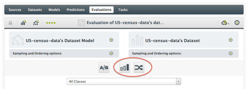
You can toggle ‘Mode’ and ‘Random’ on and off once you’ve created an evaluation, using the buttons near the top of the output area.

So even without the context of your Model, we can still give it some perspective. If either of these simple benchmarks is able to outperform your tree on a metric that’s meaningful for you, it’s back to the drawing board.

Getting Into Metrics.

Speaking of metrics, let’s talk about those for a bit.  The metrics that tell you how good your Model performs differ between classification models and regression models.

Metrics for Classification Models.

For classification models, the most familiar metric is “Accuracy“, which is simply the number of correct predictions over the number of total predictions. That sounds great, so why bother showing anything else?  Unfortunately, accuracy is easily fooled.  Suppose you have a two class model (call the classes “positive” and “negative”).  You evaluate it and it has accuracy of 99%.  What a fabulous model!  But now suppose that your test set had 990 instances of the negative class and 10 instances of the positive.  You can get 99% accuracy on this test data by just predicting negative all the time, regardless of the instance you put in!  That’s not a model, it’s a broken record. So accuracy in itself can be deceptive.

Therefor, we’ll also compute a few other metrics, that deal with skew between classes in different ways.  Let’s define some commonly used terms:  “True Positives” (TP) are the instances in the test set that have a positive class and are predicted positive by the model (so the model is right).  “False Positives” are the instances in the test set that have a negative class, but are predicted positive by the model (so the model is wrong).  “True Negatives” (TN) and “False Negatives” (FN) have similar definitions.  So for TP and TN your Model is doing great. With FP you are seeing positives where there aren’t any and with FN you are missing the positives that are there. Using those numbers, we can compute

• Precision: TP / (TP + FP); How precise were your predictions? The higher this number is, the more you were able to pin point all positives correctly. If this is a low score, you predicted a lot of positives where there were none.
• Recall: TP / (TP + FN); Did you miss a lot of positives in your predictions? If this score is high, you didn’t miss a lot of positives. But as it gets lower, you are not predicting the positives that are actually there.
• F- Measure or F1-score: 2*precision*recall / (precision + recall). This is the balanced harmonic mean of Recall and Precision, giving both metrics equal weight. At best the F-Measure is one and at worst it is zero. The higher the F-Measure is, the better.
• Phi Coefficient: See the formula here. Whereas the F-Measure doesn’t take the TN’s (explicitly) into account, the Phi Coefficient does.  Which one is appropriate depends on how much attention you want to pay to all of those negative examples you’re getting right.  If those are very important to you (as they might be in medical diagnosis), Phi may be better.  If they’re not very important (like in trying to return relevant search results), F1 is often more appropriate.

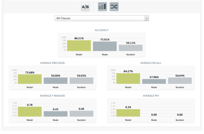
The astute reader will note that we had to pick a “positive” class to compute any of these measures.  What if we just had “Class A” and “Class B”?  Which one is positive? Luckily we don’t have to pick one. To give overall performance numbers for the Model, we simply consider each class as being positive, compute the measures and then average them together.  This is known as “macroaveraging” the measures, in the machine learning community.  So the metrics we report for all classes are “Average Recall”, “Average F-measure”, etc.  Note that below we’re showing the mode (plurality class) and random predictions as well.

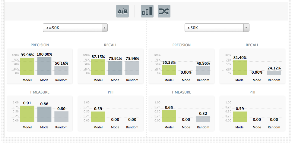
But what if you just care about the precision, or recall, or F1 score on a single class? You could be particularly interested in the outcome of one specific class, for instance if false positives of that class cost you a lot of money.  The interface allows you to call out a particular class (or pair of classes, using the A/B button) to show the performance when that class is considered the “positive” one. Below we’re seeing the performance on two classes from the census data, “Salary <= 50k per year” and “Salary > 50k per year” while, again, at the same time showing the mode and random performances per class.

Metrics for Regression Models.

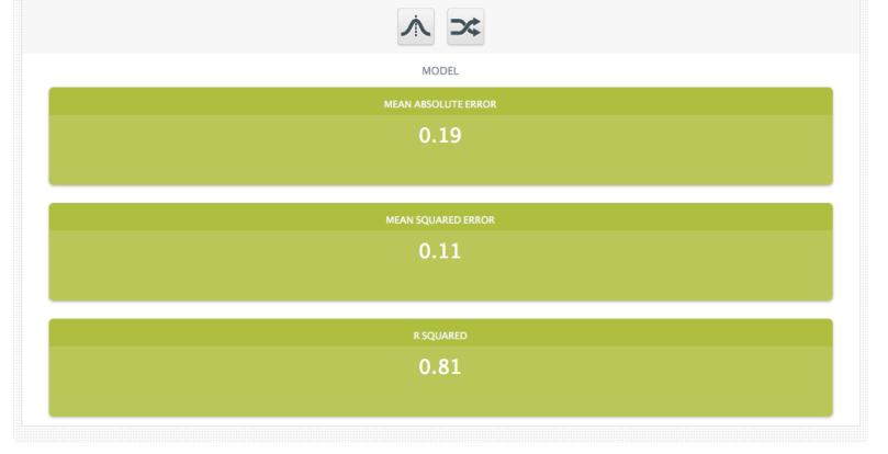
Regression models don’t have classes, so they’re a little more straightforward.  For these models the given metrics are:

• Mean Absolute Error:  The average of the absolute value of the amount by which the model misses its prediction. It tells you how close the predictions are to the actual outcomes.
• Mean Squared Error:  The average of the square of the amount by which the model misses its prediction.  Similar to the absolute error, but will obviously give a little more weight to the errors that are very large.
• R Squared: The coefficient of determination, which is essentially a measure of how much better the model’s prediction is than just predicting the mean target value all of the time. It is a value between zero and one. The closer R Squared is to zero, the closer your model is to simply choosing the mean prediction for every instance.

More to Come!

What’s that you say?  “But I don’t have a separate training and test set!  I only have one dataset!”  There’s still a way you can create a useful evaluation without splitting up the data file yourself, and we’ll go into that in Part 2.  Stay tuned!