This is the first post in a series of statistics primers to inaugurate the arrival of BigML’s new advanced statistics feature. Depending on your background as a reader, the theory portion of this post may cover ideas which you already understand. If that’s the case go ahead and skip ahead to how to access these stats in BigML. Today’s topic is Benford’s law, which can be applied to detect irregularities in numeric data. It applies to collections of numeric data whose values satisfy the following criteria:
- Have a wide distribution, spanning several orders of magnitude.
- Generated by some “natural” process, rather than, say, arbitrarily chosen by a human.
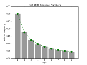
Given that those conditions are met, Benford’s law states that the first significant digits (FSDs) will be distributed in a very specific pattern. In other words, we can take each of the digits from 1 to 9 and look at the relative proportion with which they appear in the first significant position among values in the data (e.g. the FSDs for the values 122.4, -54.01, and 0.0048 are 1, 5, and 4 respectively). If these proportions match the ones predicted by Benford’s law, then we can be assured that our data satisfy our two criteria. Otherwise, the data may have been tampered with, or may simply cover too narrow of a range for Benford’s law to apply. If we denote pd as the proportion of the data in which the digit d is in the first significant position, Benford’s law states that these proportions will take on the following values:

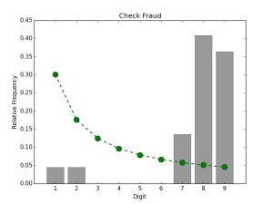
In the plots that follow, p1 through p9 are drawn as the green line. We see that 1 should be the FSD in about 30% of the data while 9 should only be about 6% of the FSDs. The first two plots are examples of numeric data which conform to Benford’s law. The Fibonacci numbers and US county populations both satisfy the criteria given above. The gray bars denote the relative proportions of FSDs in the data.

The next two plots are examples of non-conforming data. The first example is data from the ubiquitous Iris dataset. Although it is undeniably a natural dataset, it fails the first criterion, since its values span only the the narrow range from 4-8 cm. The second example is an instance of fraudulent data. As chronicled in the State of Arizona v. Wayne James Nelson (CV92-18841), Mr. Nelson, a manager in the Arizona state treasurer’s office, attempted to embezzle nearly $2 million through bogus vendor payments. Since Nelson started small and worked his way up to larger amounts, the values do satisfy the first criterion. However, as all the amounts were artificially invented, the second criterion is not satisfied and the final FSD distribution is very far from the one given by Benford’s law, with the digits 1-6 being too scarce and 7-9 being much more common than expected.

The last of these examples highlights the potential usefulness of this phenomenon in detecting suspicious numbers, and indeed there are many documented cases where fraudulent data have been exposed through application of Benford’s law. Multiple analyses of results from the 2009 Iranian presidential elections have used Benford’s law to provide statistical evidence suggesting vote rigging. A post mortem Benford’s law analysis of the accounts for several bankrupt US municipalities revealed inconsistent figures, which could be indicative of the fiscal dishonesty which led to the municipalities’ financial ruin. A team of German economists applied a Benford’s law analysis to the accounting statistics reported by European Union member and candidate nations during the years leading up to the 2010 EU sovereign debt crisis. They found that the numbers released by Greece showed the highest degree of deviation from the expected Benford’s law distribution. As Greek national debt was one of the main drivers of the crisis, we can draw the conclusion that the Greek government was fudging the numbers to hide its fiscal instability. Interestingly, while researching this topic we found that the Greek source data for this analysis is now conspicuously absent from EUROSTAT website.
Testing Benford’s Law
Having seen that deviation from Benford’s law can be a useful indicator of anomalous data, we are left with the question of actually quantifying that deviation. This brings us to the topic of statistical hypothesis testing, in which we seek to confirm or reject some hypotheses about a random process, given a finite number of observations from that process. For the purposes of our current discussion, the random process in question is the population from which our numeric data are drawn, and the hypotheses we consider are as follows:
H0 (null hypothesis): The population’s FSD distribution conforms to Benford’s Law
H1 (alternate hypothesis): The popluation’s FSD distribution is different from Benford’s Law
Depending on the outcome of the test, we either accept the null hypothesis, or reject it in favor of the alternate hypothesis. In the latter case, we may have grounds for applying more scrutiny to the values as failure to fit Benford’s law can be a sign of questionable data. The second piece of a statistical test is a significance level, also known as a p-value. In statistics, the results we obtain are not concrete facts; rather, our conclusions are parameterized by some level of certainty less than 100%. The precise definition of the p-value is rather nuanced, but we can think of it as how extreme the calculated test statistic is, under the assumption that the null hypothesis is true. The workflow of a statistical test is thus as follows:
- Calculate a test statistic from the sample data, using the method prescribed for the specific test.
- Choose a desired significance level, which determines a critical value for the test statistic.
- If the calculated statistic is greater than the critical value, then the null hypothesis is rejected at the chosen significance level. Otherwise, the null hypothesis is accepted.
For Benford’s Law hypothesis testing, commonly employed tests are Pearson’s Chi Square test-of-fit, and the Cho-Gaines d statistic. Let’s work these tests out using our four example datasets.
Chi Square Test-of-fit
This test is a general purpose test for verifying whether data are distributed according to any arbitrary distribution. The test statistic is computed from counts rather than proportions. Let
be the observed proportion of digit d in the data’s FSD distribution, and
be the expected Benford’s law proportion defined previously. For a data set containing N observations, the observed and expected frequencies are given by
and
respectively. The Chi-square statistic is defined as follows:
The critical value for this test comes from a chi-square distribution with (9-1) = 8 degrees of freedom. For a significance level of 0.01, we get a critical value of 20.09. If the value of χ2 is greater than this value, then we can reject a fit to Benford’s law with 99% certainty. In the Nelson check fraud dataset, we have the following observed frequencies:
In other words, 1 was the first significant digit in one of the entries, while 9 was the FSD in 8 entries. For this 22 point dataset, our expected Benford’s law frequencies are:
Computing the chi-square statistic is a simple matter of plugging in the values:
The obtained value is greater than the critical value, so we can indeed say that the fraudulent check data do not fit Benford’s Law. Iris, our other non-conforming dataset also produces a chi-square statistic larger than the critical value (506.3930), while the Fibonacci and US Census datasets produce values less than the critical value (0.1985 and 10.6314 respectively).
Cho-Gaines d
For small sample sizes, the chi-square test can encounter difficulty in discriminating between data which do and do not fit Benford’s Law. The Cho-Gaines’ d statistic is an alternative test which is formulated to be less sensitive to sample size. It is defined as follows:
For a significance level of 0.01, the critical value for d is 1.569. The values for d from our example data are 0.114, 1.066, 7.124, and 2.789 for the Fibonacci, US Counties, Iris, and Nelson datasets respectively. The first two values are less than the critical value, whereas the last two are greater, thus producing a result which is consistent with the chi-square test and visual comparison of the FSD distributions. Rather than being computed from a well parameterized distribution like the chi-square test, these critical values for the Cho-Gaines’ d test are obtained from Monte Carlo simulations, and are only available for a few select significance levels. This means that it is not possible to know the exact p-value for any arbitrary value of d, and thus represents a tradeoff compared to the chi-square test.
Wrap-Up
In this post, we’ve explored First Significant Digit analysis with Benford’s Law. This straightforward concept, when combined with simple statistical tests, can be a useful indicator for rooting out anomalous numeric data. Benford’s law analysis is one of the many statistical analysis tools that are being incorporated into BigML. So stay tuned for a follow up post on how to perform this handy task and more on BigML.
